
Now that we have defined the alliance index to quantify the relationship between castaways, what can we do next? We can build a Survivor alliance network by taking castaways as nodes and the alliance index between a pair of castaways as the edge. The Survivor alliance networks can then be used as a visual summary of the relationships in every season. In this post, I’ll demonstrate how we can construct alliance networks and then show what they look like.
Survivor Alliance Networks
Let’s focus on a single season of Survivor. We can represent this season with a network by considering the castaways as our set of nodes and the alliance index between each pair of castaways as the set of edges. Note that our interpretation of the alliance index is relationship strength, so the resulting network is not just a plain, unweighted network, but a weighted network with relationship strength given by the alliance index. Later on, we will visualize relationship strength with edge thickness.
We can use the NetworkX module in Python to build the network in a really easy manner. In order to define a network in NetworkX, we construct a network object using nx.Graph(). Let’s call the resulting network G. To add nodes to G, we do G.add_nodes_from(node_list) where node_list is, naturally, the list of nodes. To add an edge to G, we do G.add_edge(edge_pair) where edge_pair is a pair of nodes we want to connect.
We then define a function plot_network() which takes as input the season name and outputs the network of relationships as a png file. This function relies on the scraping code and the alliance index code from Scraping the Survivor Wiki and Computational Analysis of Survivor Alliances, respectively. We set the top relationships parameters m to 50 and number of voting rounds filter to 3 by default. To arrange the nodes in space, we use the spring layout since it accentuates clustering of nodes.
num = dict(zip(seasons,range(1,len(seasons)+1)))

def plot_network(season_name,m=50,k=3):
    """
        Plot the network of alliances for season_name.
        Inputs:
            season_name : string, name of season
            m           : top relationships to consider
            k           : filter for number of voting rounds
    """
    url = turn_to_url(season_name)
    dd = extract_voting_table_as_df(url)
    top_m = return_top_m_relationships(dd, m, k)

    sns.set_style("white")
    G=nx.Graph()

    with_edge = []
    for i in dd.index:
        for tup in top_m.index:
            if i in tup:
                with_edge.append(i)
                break
    # set castaways as nodes
    G.add_nodes_from(with_edge)

    coral=(255./255, 127./255, 80./255)
    for i in range(len(top_m.index)):
        # use alliance index as edge weight
        G.add_edge(top_m.index[i][0], top_m.index[i][1], weight=top_m.values[i])

    pos = nx.spring_layout(G)
    nx.draw_networkx_nodes(G,pos,node_color = coral,node_size=1500)
    nx.draw_networkx_labels(G,pos,font_size=18)
    weights = [5*G[u][v]['weight'] for u,v in G.edges()]
    nx.draw_networkx_edges(G,pos,width=weights,alpha= 0.7,edge_color = 'gray')
    plt.title('{}'.format(season_name),size=40)

    fig = plt.gcf()
    fig.set_size_inches(10,6)
    ax = plt.gca()
    ax.axis('off')

    plt.tick_params(
        axis='both',
        which='both',      # both major and minor ticks are affected
        bottom='off',      # ticks along the bottom edge are off
        left='off',         # ticks along the top edge are off
        labelbottom='off',
        labelleft='off') # labels along the bottom edge are off

    plt.savefig('networks/{}_{}_network_top_{}_filter_{}.png'.format(num[season_name],season_name,m,k))
Using the function defined above, we can plot the network for each Survivor season using the following for loop:
seasons = ['Borneo', 'The Australian Outback', 'Africa', 'Marquesas', 'Thailand', 'The Amazon',
           'Pearl Islands', 'All-Stars', 'Vanuatu', 'Palau', 'Guatemala', 'Panama',
           'Cook Islands', 'Fiji', 'China', 'Micronesia', 'Gabon', 'Tocantins', 'Samoa',
           'Heroes vs. Villains', 'Nicaragua', 'Redemption Island', 'South Pacific',
           'One World', 'Philippines', 'Caramoan', 'Cagayan', 'San Juan del Sur',
           'Worlds Apart', 'Cambodia', 'Kaôh Rōng', 'Millennials vs. Gen X']

for season in seasons:
    plot_network(season)
Let’s look at the Survivor alliance network of several past seasons of Survivor.
First, let me give three notes.
- Remember that edge thickness denotes the alliance index (or the strength of the relationship). A thicker edge corresponds to a higher alliance index, while a thinner edge corresponds to a lower alliance index.
- More often than not, pre-merge boots do not appear in the alliance networks since they get filtered out by the parameter k.
- The alliance networks are a function of m and k. For our analysis, we focus solely on the case m=50 and k=3. Changing m and k will give different results.
I don’t want to flood this post with networks. If you’re interested in seeing the networks, check out my Github
I haven’t watched every season of the show, so I can’t give a detailed analysis of every network.
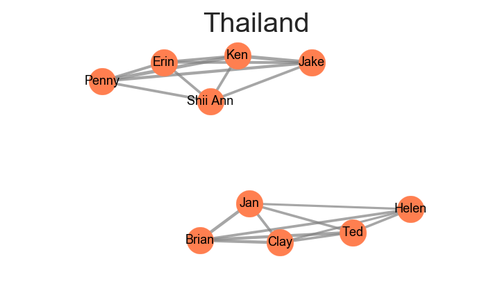
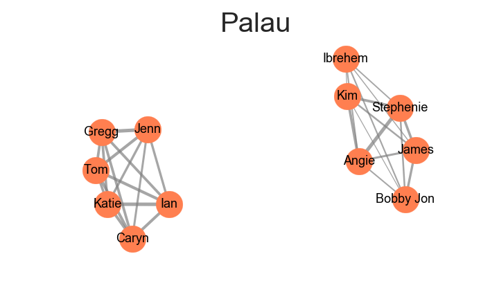
One thing I noticed is that there are some seasons which have distinct, non-connected clusters (Thailand and Palau)
while some seasons have a single, connected cluster (Worlds Apart and Cambodia).
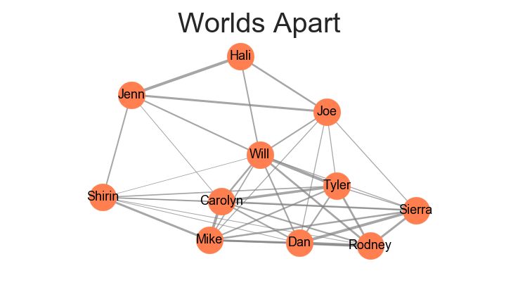
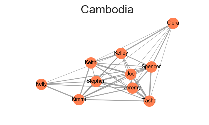
There are seasons wherein alliances lines are drawn from the get-go, whereas in other seasons alliances are much more fluid and can change from one tribal council to the next.
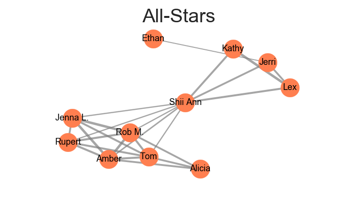
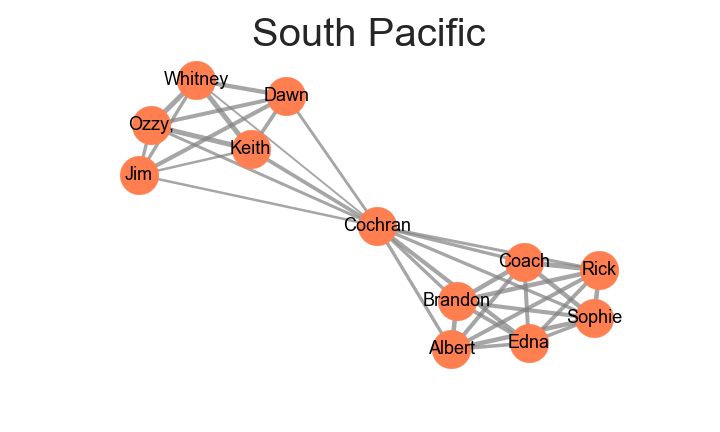
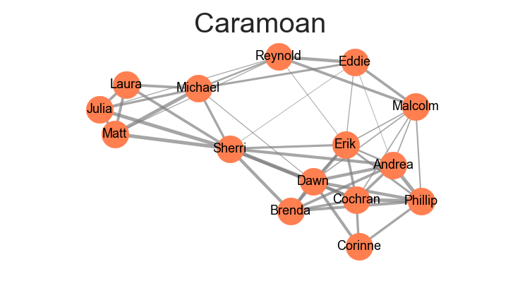
The alliance networks highlight situations wherein a castaway had two distinct alliances during the season, perhaps one pre-merge and one post-merge, or if the castaway flipped on his alliance. This can be seen with Shii-Ann in All-Stars,
Cochran in South Pacific,
and Sherri in Caramoan.
So what is the point of these networks? Apart from them being nice to look at, the alliance networks that we created summarize the relationships of each season of the show in a neat image.
Caveats
- One major issue I have with the networks we have made is that time element gets removed from the equation. We all know that Survivor alliances are dynamic. That is, they change over time. Heck, they may even change several times within an episode! An interesting project we can do in the future is to look at the time-dynamics of the alliance network. In other words, we look at how the network of relationships change over each voting round, from the first tribal to the pre-final boot.
- Survivor Blood vs. Water is breaking my algorithm for some reason. I’m getting a key error with Gervase, and I don’t really want to deal with it right now.
Network Analysis of Survivor Analaysis
The next thing I’m going to do is compare the different seasons of Survivor using some network metrics. This will hopefully enable us to contrast the different seasons of Survivor from one another.
But First, a Primer on Metrics
By representing phenomena as networks, we can study the mathematical properties of their structure. Typically, in network analysis, we quantify properties using network metrics. These network metrics are developed to answer specific questions. For example, we can ask which nodes are the most important in the network. The metrics which answer this type of question are called centrality metrics. The three most common centrality metrics are degree, closeness and betweenness. In the context of social networks, one question we can ask is whether our friends are friends of one another as well. The clustering coefficient was developed to answer this question.
How many friends do you have?
Degree. The degree of a node is the number of edges connected to it. It is a measure of how many relationships the node has.
In the case of Facebook, degree is the number of friends that a user has. Degree only considers the friends of a certain user and doesn’t really take into account the Facebook network as a whole. Because of this, degree is considered as a local metric. A user who has high degree we can think of as a local celebrity — he has lots of connections in his sphere of influence, but not necessarily outside of it.
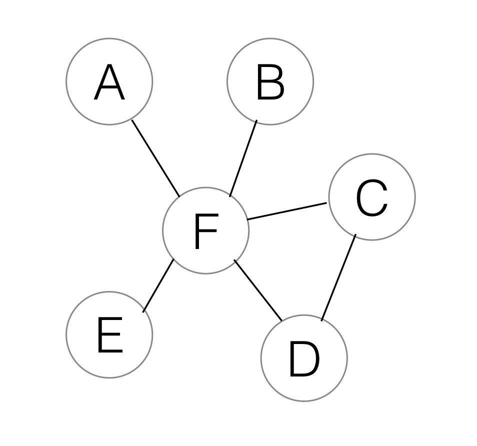
The node F is the node with the highest degree in the network, since it is connected to everyone else, whereas A, B, and E have the lowest, since each only has one connection, F.
How near are you to everyone else?
Closeness. The closeness of a node is defined as the inverse of its farness, where farness is defined as the sum of the distances of the shortest paths from the node to every other node in the network. A node which has high closeness requires very little travel time to get to other nodes in the network.
Since we need to calculate shortest paths between every node pair in the network, closeness is, as opposed to degree, considered a global metric. Every node in the network needs to be considered to compute it.
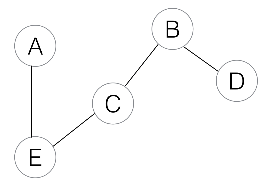
Node C has the highest closeness in the network. Since C is at the midpoint of the linear network, it has the smallest average distance to every node in the network. On the other hand, A and D are at the ends of the line, and so their average distance to the other nodes is at the maximum.
How often do you connect other people?
Betweenness. The betweenness of a node is defined as the number of shortest paths (of every other node in the network) that passes through it. Intuitively, we can think of a node with high betweenness as a bottleneck connecting two or more large collections of nodes with one another. Removing a node with high betweenness from the network will often divide the network into disjoint subnetworks.
Again, betweenness is a global metric since it requires the calculation of shortest paths.
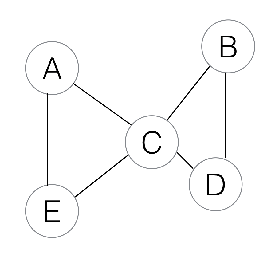
Node C has the highest betweenness here, since the shortest paths from {A,E} to {B,D} need to go through C. On the other hand, no shortest path passes through any other node in the network.
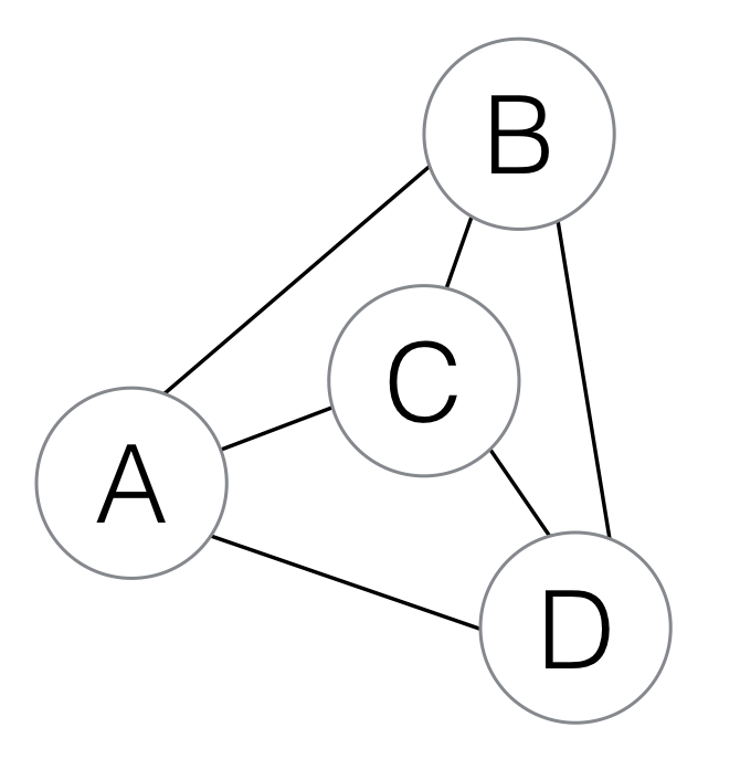
Node C has high closeness and low betweenness, since the shortest path from C to any other node is one, while the shortest path between nodes other than C do not pass through C.
Are your friends acquainted with one another?
Clustering. To calculate the clustering coefficient of a node, we look at all other nodes connected to the specified node, and count the number of edges which exist among the node’s neighbors. The clustering coefficient is a measure of how connected the node’s neighbors are — do they cluster around the node?
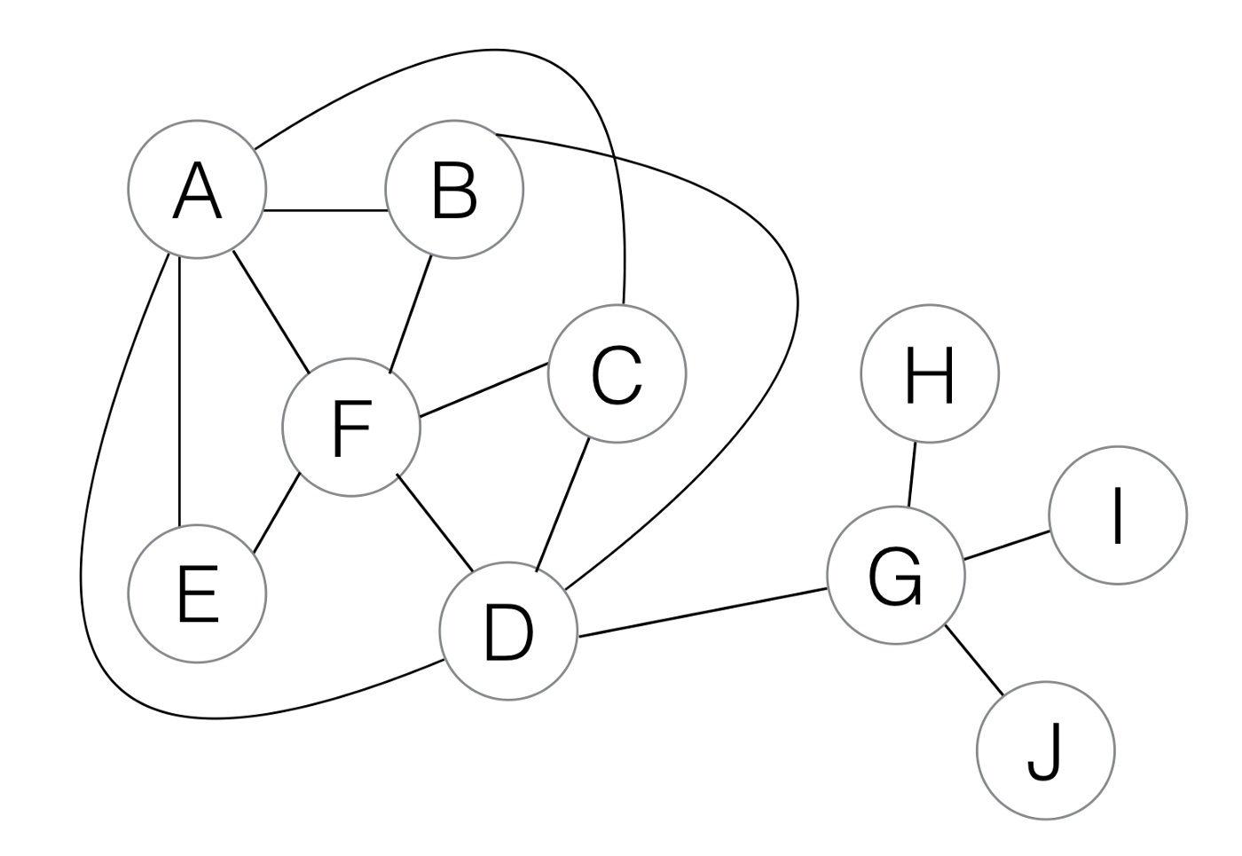
Node F has high clustering. The majority of F’s neighbors are connected amongst themselves. The opposite happens with node G, wherein none of his neighbors are connected.
Some Notes
All of the metrics defined above refer to a specific node in the network. We can also associate a metric to the whole network. How do we do this? By averaging the metric over all the nodes in the network.
Usually, the metrics presented above are normalized to be in the range 0 to 1, that is from weakest to strongest. A degree of 1 says that the node is connected to every other node in the network. A clustering coefficient of 1 means that all the neighbors of the node are connected to one another.
Taking it one step further, networks sometimes have added information in the form of edge weights. These edge weights quantify the strength of relationship represented by the edge. These edge weights can be included in the calculation of degree, closeness, and betweenness by setting the distance between two nodes as the corresponding edge weight.
Survivor Network Metrics
We calculate some standard metrics of Survivor alliance networks, namely the centrality metrics degree, closeness and betweenness and the clustering metric. This will hopefully enable us to compare and contrast the different seasons of Survivor.
There are two ways we can approach network analysis. First, we can perform an intranetwork analysis, comparing nodes belonging to the same network. Second, we can perform an internetwork analysis, comparing two or more different networks with one another. Our approach in this blog post is the second one, as our goal is to compare and contrast the different seasons of Survivor.
We will use four metrics to perform network analysis, as we have introduced above: degree, closeness, betweenness, and clustering. The first three metrics are all considered as centrality metrics, since they measure how important nodes are in the network. These metrics are used, for example, to determine the most influential person in a social network. The fourth metric, clustering, is a measure of the density of ties around a node, i.e. how likely your friends are friends of each other.
We calculate the metrics in two different ways. First, we will look at the average value of the metric over the whole network. In other words, we average the metric over all castaways in the alliance network. Second, we look at the maximum of the metric over all nodes or castaways.
Note: Our calculations for the centrality metrics are alliance-index-weighted, while the clustering metric is not.
Average Metrics
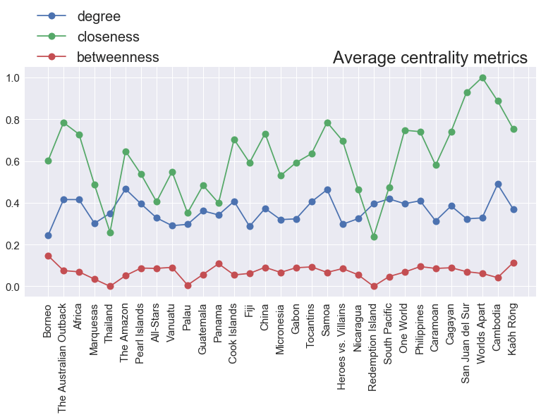
The Amazon, Samoa and Cambodia have the top three largest average degree, while Borneo has the smallest one. A castaway with a high degree is someone who has voted with a lot of other castaways, so that means that a season with high average degree is one whose castaways have worked with almost everyone, regardless of alliance lines.
In terms of average closeness, Worlds Apart has the largest one and Thailand, Palau and RI have the smallest. Intuitively, closeness can be thought of as how tight the alliance network is. A season with large average closeness is one wherein the castaways are all ‘close’ to one another.
For betweenness, Borneo reigns supreme and, again, Thailand, Palau and RI lag behind. A node with high betweenness is one which acts as a bottleneck between disconnected clusters. That is, to go from one location in the network to another, the path must go through the node. So in this case we see that the three with the lowest ones coincide with the networks with disconnected clusters since no node acts as a bottleneck.
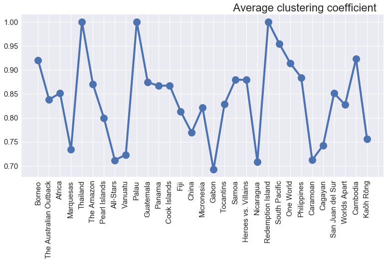
Some seasons have large average clustering coefficient, while some have a small one. The ones with the large clustering coefficient coincide with those with disconnected clusters that are almost complete or fully connected — Thailand, Palau and Redemption Island. The ones with small clustering are those which are more homogeneously spread out like Gabon and Nicaragua. Clustering basically measures the formation of cliques. In this case, we can think of seasons with high clustering as having tight alliances and those with small clustering as having fluid ones.
Maximum Metrics
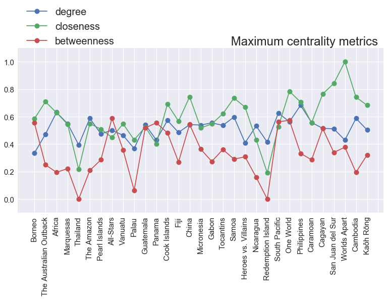
A season with large maximum degree is one which has a castaway that was almost everyone at one point or another in the season. In this case, Africa and Philippines are on top.
For maximum closeness, we see that Worlds Apart, again, is on top and Thailand and RI are on the bottom. In the case of maximum betweenness, All Stars, South Pacific and One World rank highest, since in each of those there is/are a bottleneck castaway/s (Shii-Ann, Cochran, Tarzan/Troyzan) which connects all others.
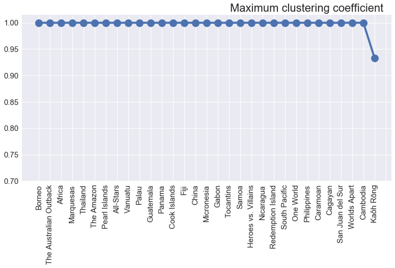
Every season has a castaway with perfect clustering, except for Kaoh Rong (well, it’s not really significant, since it’s still at 0.95). This means that there’s someone in every season whose neighbors in the alliance network are all connected as well, which is basically what an alliance is.
