
Recently I’ve been getting my feet wet with Bayesian statistics. To reinforce my understanding, I decided to apply the concept to Survivor in order to compare the contestants’ hit rate. By hit rate, what I mean is how often a contestant’s vote at tribal council contributed to the elimination of another contestant.
The hit rate is an indicator of a contestant’s awareness of tribe dynamics, as a high value indicates that he is always in-the-know and consequently knows where the votes are going.
Computing the hit rate as a simple ratio of successes to number of tribal councils is problematic. Evidence volume is imbalanced, i.e. some contestants were able to go deep in the game and had a lot of opportunites to vote, while some contestants unfortunately did not, so their voting records have lots to be desired (from a statistics viewpoint).
In concrete terms, estimating the hit rate for successful contestants can be done in a reliable manner by getting the ratio of successful votes to the number of tribal councils attended. However, this cannot be done reliably for early boots. For instance, pre-merge boots wouldn’t have a lot of statistics, especially first boots as they would just register a 0 percent hit rate.
But a 0 percent hit rate is not a good estimator of the hit rate for the first boot, as it’s basically putting him at the same level as a contestant who, for example, attended 10 tribal councils and voted incorrectly for all of them. One could argue that the second person should have a lower hit rate because of the level of evidence presented. Between 0/1 and 0/10, the latter is a stronger 0% as there were more opportunities for the latter contestant to fuck it up and he actually did, while the former unfortunately had one. A question to ask for the first contestant is: Was it a fluke? So it’s safe to say that there is much more uncertainty in the 0/1 0% hit rate than the 0/10 0% hit rate.

At the opposite end, between a contestant with a 1/1 100% hit rate (which is possible, as in the case of Neal in Kaôh Rōng who was evacuated after his first tribal council, where he voted correctly) and a contestant with a 14/14 100% hit rate, there is much more uncertainty in the first one as there is very little evidence available.
It gets ambiguous when presented with ratios of different levels of evidence. Is a 1/4 or a 0/1 worse? Is a 10/13 or a 11/14 better? There has to be a framework wherein we can put all of these in a single scale.
Thinking of the hit rate as a point value (ex. 0%, 20%, 30%) doesn’t facilitate comparison of uncertainty in a very natural manner, and as we saw earlier, uncertainty is an important measure to consider as an indicator of the level of available evidence.
An alternative way we can think of the hit rate (that fits in naturally with uncertainty considerations) is by treating it as a probability distribution.
Allow me to elaborate.
We can think of the hit rate as an inherent trait of a contestant - some may have a high hit rate because of hightened social awareness, while some may have a low one because of being a natural blabbermouth. A reasonable assumption that we can make is that the hit rate is a property drawn from some distribution common to all players.
By going with this assumption, we have an added bonus: information from each player affects estimates of the hit rate of all other players indirectly as we are assuming that all of the players draw their hit rate from a common distribution. So a 0/2 hit record of a contestant will not translate into a 0% hit rate since we also look at the average statistics of everyone in consideration before giving an estimate. A better estimate would be something close but lower to the overall hit rate and with high uncertainty, as there is very little evidence in a 0/2 hit record. This property of Bayesian models is called Bayesian shrinkage, because there is a tendency to converge to the mean, which is not a bad thing as it leads to more stable inference.

A One-Level Hierarchical Model
For the base case, let’s look at a simple one-level hierarchical model.
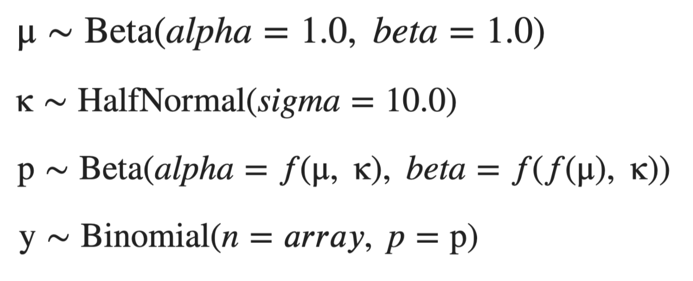
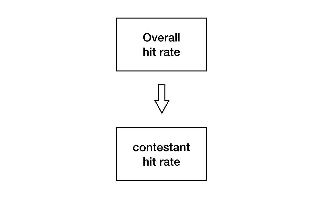
where we interpret y as the number of hits and p as the hit rate. f's are chosen such that mu and kappa can be interpreted as the mean and concentration of p, respectively. In this one-level model, we think of the hit rate p for each player as a distribution whose mean is drawn from a shared distribution of hit rates that we estimate concurrently with the individual player hit rates. In a simple diagram, we have:
I used pymc3 and all available data from seasons 1 to 39 to train this hierarchical model. The KDEs and traces for themu and kappa posteriors are shown below.
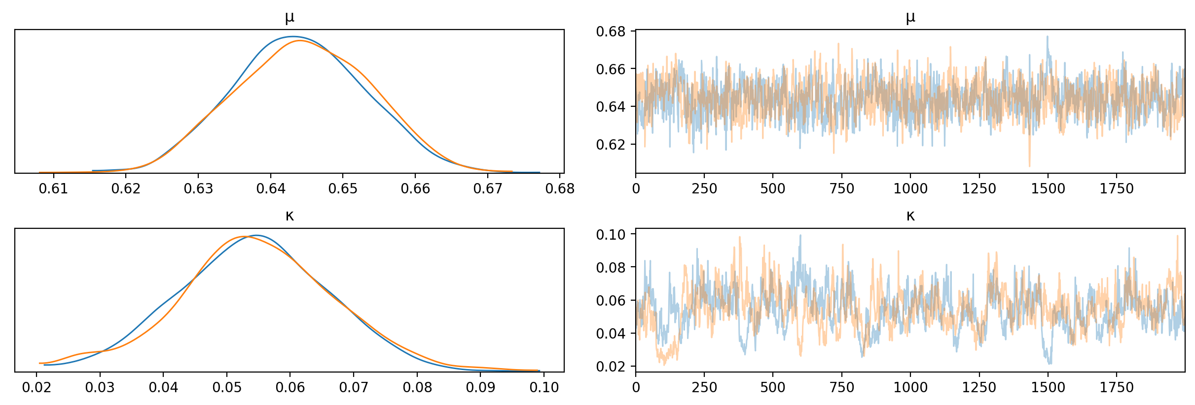
What do these mean? mu is the mean of the overall distribution from which we draw individual player means, so mu represents an overall mean of all players. This means that ~64% is an estimate of the hit rate of an average contestant, and a credible range which represents our uncertainty in the value is 62% to 67%. kappa is the concentration of the overall distribution and represents how spread out the distribution is around mu. ~5%, not really that big.
Case Study: Island of the Idols
Let’s take the latest season Island of the Idols as a case study. Let’s look at the hit rate distributions of all players and sort by the median, top to bottom.
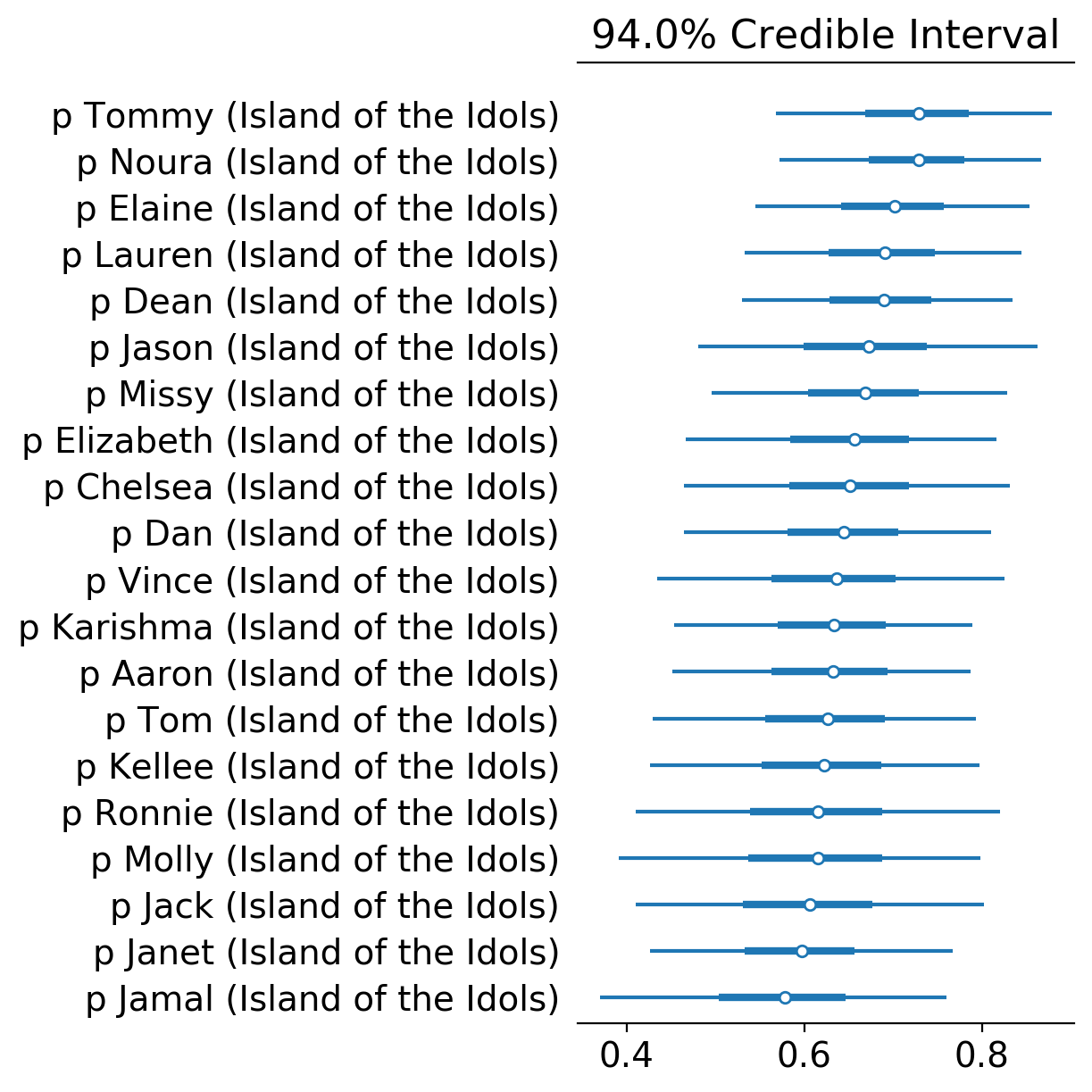
Funny to see that Noura (8/9), together with the season’s winner Tommy (8/9), has the highest median hit rate across all contestants. Obviously, the hit rate is not an indicator of winnability as Noura probably has the lowest chance of winning the game that season apart from Dan.

Interesting to see Janet (5/10) near the bottom of the list as she finished 5th while Kellee (2/4), the merge boot, ranking higher than her based on hit rate median. The high level of evidence Janet presented (10 votes) allowed her to pull away from the overall mean (~64%) more than Kellee (5 votes), which added proof of her being worse than Kellee in terms of hits. Also note the credible interval for Kellee is wider than that of Janet’s since Janet has a lot more data to work with.
Ronnie (0/1) and Molly (0/1), the first boots, appear near the bottom of the list, with medians lower than the overall mean and with very wide credible intervals, since there isn’t a lot of data to work on for the pair.
Case Study: All-Time Rankings
Now let’s look at the top 20 and bottom 20 Survivor contestants in terms of estimated Bayesian hit rate.
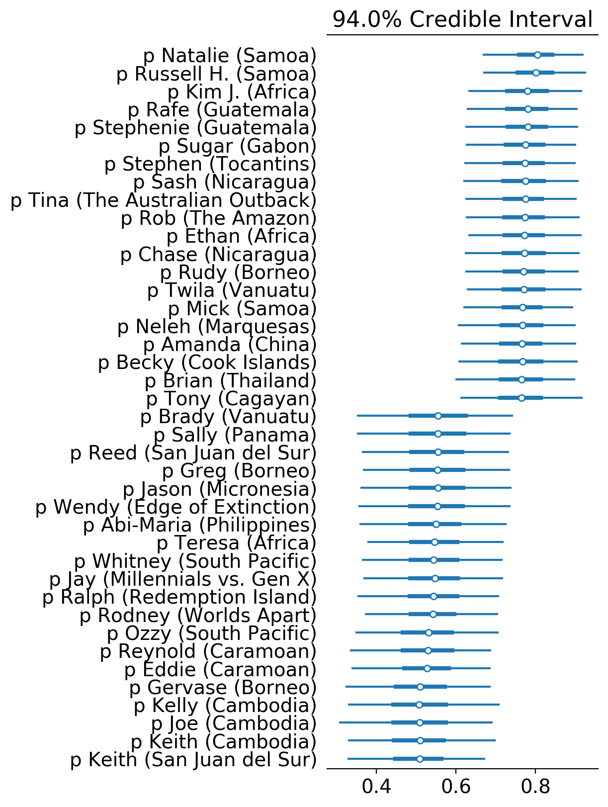
The duo Natalie White and Russel Hantz from Samoa impressively top the list, Kim Johnson from Africa ranking third, and another pair Rafe Judkins and Stephanie LaGrossa from Guatemala rounding up the top 5. Interesting to see two pairs at the top of the list. Alert: power duos are a thing.
Funnily, at the other end of the list are Keith Nale’s two games (Cambodia and San Juan del Sur). Though he was able to go deep in the game in both seasons, he was always in an underdog and, dare I say, a clueless position. Some Cambodia buddies also appear in the bottom: Joe and Kelly. Caramoan buddies Eddie and Reynold round out the bottom 5.

In a way, low hit rate can be an indicator of underdog status as it signifies a high rate of being on the wrong side of the votes.
Case Study: Winners
Zooming in only on winners, we have the following forest plot.
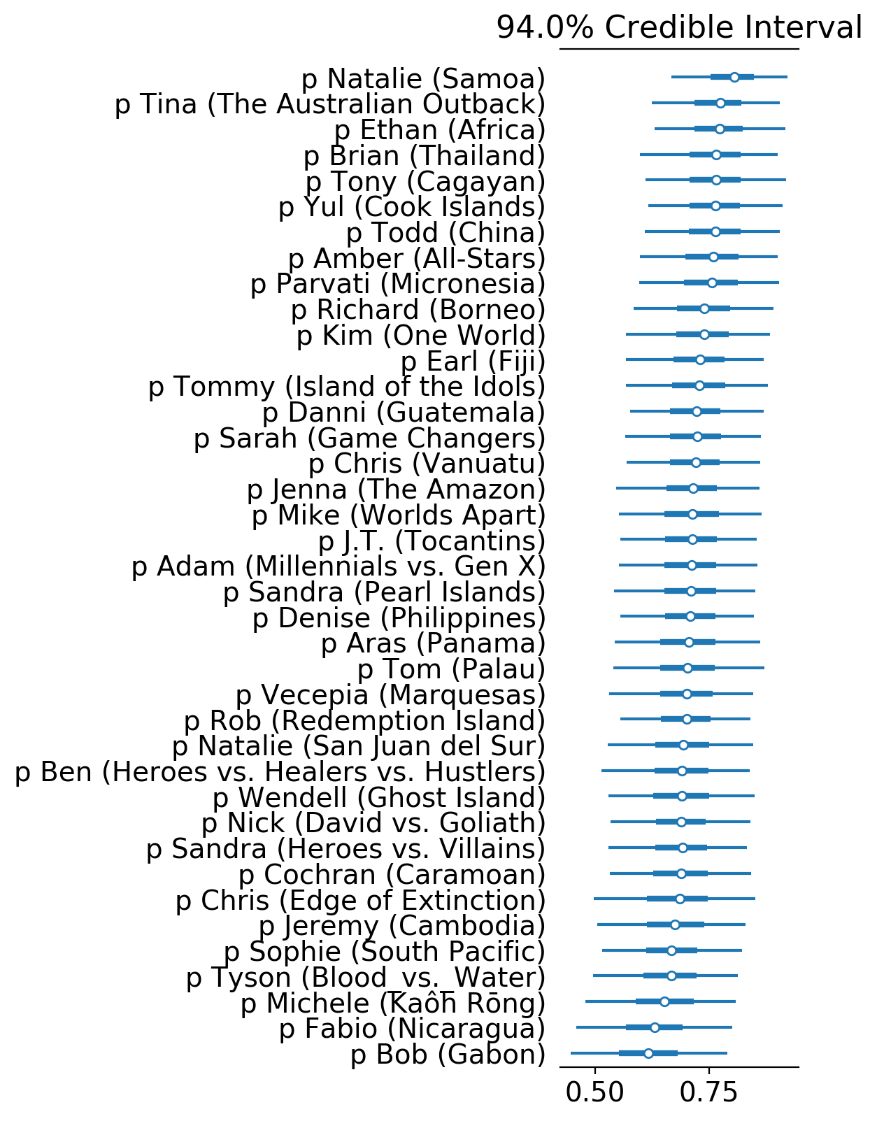
Natalie, Ethan and Tina are top 3, while Bob, Fabio and Michele are bottom 3. It’s very easy to discern the difference in gameplay of the top and bottom rankers. The ones on top were part of a dominating alliance and smooth path to the end, while those on the bottom had a difficult and rocky path.
A Two-Level Hierarchical Model
Now let’s focus on two seasons: Cagayan and Kaôh Rōng. What do these two seasons have in common? The theme: Brains vs Brawns vs Beauty. As this tribal division is a categorization of the players, we can add this as another level in our hierarchical model.

While in our one-level hierarchical model the mean of the hit rate of a player is drawn from an overall distribution, in our two-level hierarchical model the mean is drawn from one of three distributions, with the choice dependent on which tribe the player belongs to (Brains, Brawns, or Breauty).
In pictures, we have:
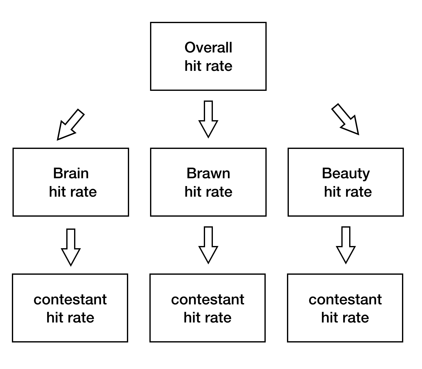
Since we have three additional distributions, one for each tribe, we can peruse tribe-level hit rates in addition to player-level hit rates.
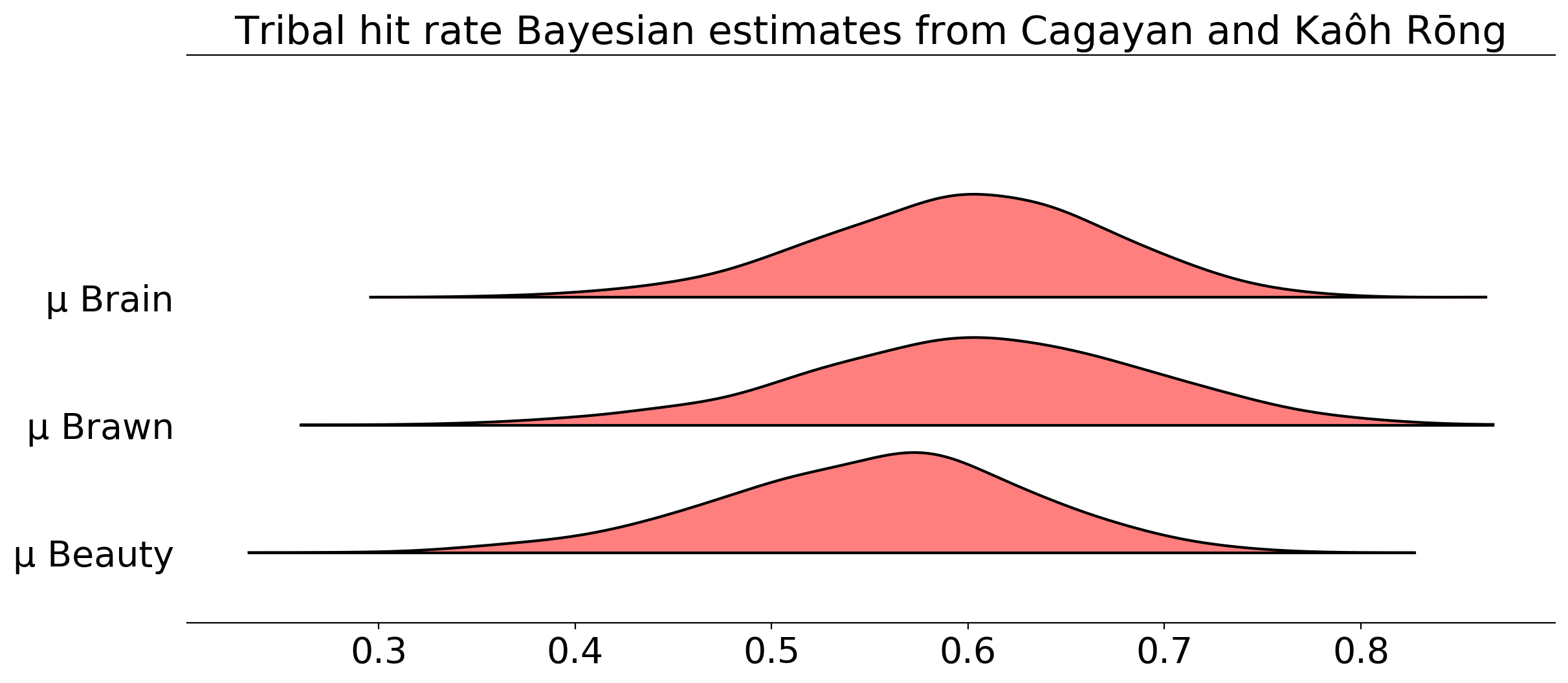
Here, mu represents the mean of the tribe-level distribution. What this plot is telling us is that the mean hit rate of the three tribes are very similar to one another, with Brains and Brawns more similar to one another than Beauty, and that the Beauty median is a bit lower than the other two. Uncertainty considered, not much difference across the three tribes, but if I were to put money on which player would vote correctly, I’d put money on someone from Brains/Brawns than Beauty based on the analysis.
Summary and Improvements
So what have we done in this analysis?
First, we were able to estimate the hit rate of each player not just as a single point estimate but as a a distribution that encodes our uncertainty, which in turn is based on the level of evidence we have on each player. In addition, our estimates are not just simple ratios which ignore other contestants’ information, instead we pool hit rate information from all other contestants to inform estimates for each player.
Using the one-level hierarchical model over all players, we were able to find out the most and least successful contestants (in terms of voting). We also made an observation regarding the existence of power duos and loser duos based on the ranking, as well as the hit rate being a possible indicator of underdog status.
Second, by adding another layer in our hierarchical model, we examined tribe categorization (Brains vs. Brawns vs Beauty) to estimate tribal hit rates. We saw that Brains and Brawns were very similar in distribution, while Beauty lags a bit behind.
So far, so good. However, there’s a lot more to be desired in terms of model performance. For the considerations below, we only look at the one-level hierarchical model over all players.
Let’s compare raw hit rate ratios with our Bayesian estimates.
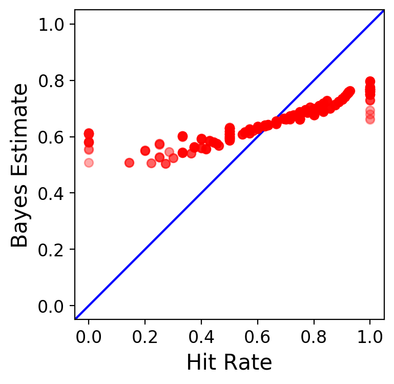
In the plot, each red dot represents a player, and the blue line shows the identity function. At first glance, you can see how strong Bayesian shrinkage has affected all parameter estimates. Low hit ratios were pulled up towards the overall mean, while high hit ratios were pulled down. The level of evidence dictates how strong the pull is: the less evidence, the weaker; the more, the stronger.
If we want to combat this strong Bayesian shrinkage, we would need more evidence for our players, as the low level of evidence across the board necessitates a strong reliance on the overall mean.
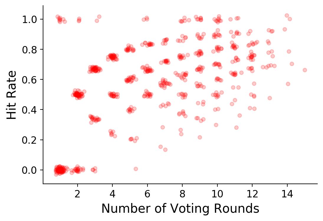
Looking at the graph above, it is apparent that the hit rate and number of voting rounds have some positive relationship. Thinking about it, it makes sense as a higher hit rate could indicate that a player is more socially aware, in turn allowing him to survive more votes. This relationship isn’t contained in our model, and it might be interesting if we could directly encode this positive relationship, as well as demographic considerations… leading us to the realm of Bayesian regression.