
I’ve been playing around with survival analysis at work, and it occurred to me that Survivor is the perfect case study for the topic since it deals with people metaphorically dying when they get voted out.

Let’s formulate some interesting questions that survival analysis can answer:
- How do demographic variables (age, sex, location) relate with chances of reaching day 39?
- Is there any difference in survivability in old-school Survivor vs new-school Survivor? (Sorry, only Survivor fans will be able to relate!)
The attack here is to graph survival curves for each value of the demographic variables. The survival curves estimate the probability of reaching day 2, day 3, up to the final day, day 39. Comparing the survival curves for different values of age, sex, and location would be our approach moving forward.
First of all, let me give a brief rundown on what survival analysis is.
Survival Analysis and Kaplan-Meier Curves
When will I die? When will I recover from my sickness? When will the customer stop using our company’s service? These are questions that survival analysis attempts to answer in a probabilistic sense.
There are two common elements across the mentioned probelms: a time element (which answers when) and the event itself (which answers what will happen). One of the main objectives of survival analysis is to map time t to the probability of existing up to time t. This function, called the survival function often denoted by S(t), is usually presented as a graph called the survival curve.
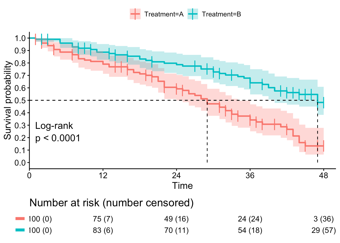
Survival curves are really handy since they can be used to answer a ton of interesting questions. Take for example the scenario of disease treatment. Let’s say we have two different treatments A and B. We can look at the survival curves for A and B to see which treatment is more effective — the one with the higher survival function consistently across time is obviously the better option.
But how do you actually construct a survival function?
Estimation can be done by conducting an experiment. In harsher terms, we observe subjects from the start event up to the time that they die. Ideally, we would know the time of death of ALL our subjects, and in that case we can empirically construct the survival curve by simply counting the number of subjects still alive at time t, for every t possible.
But there are cases when the observation period of the experiment completes — meaning we aren’t tracking the subject anymore — but some subjects are still alive. Or there might be cases wherein we lose track of still-alive subjects during the experiment, and therefore we don’t know the actual time that they die. All we know is that they’re alive up to the point wherein we last saw them. These last two scenarios are called right-censored observations since the time of death (or the time of event in survival analysis terms) is censored, meaning we don’t know the specific time of death but we have limited info on it.
How do we construct survival curves in this case?
We can construct Kaplan-Meier (KM) survival curves. The basic idea is to use all available information for each subject, even right-censored observations, up until they die or are censored, and then use the chain rule for conditional probabilities to tie up all the pieces of information together. In this way, we are able to use censored data even if we don’t know the actual time-to-event. You can read more about KM curves on Wikipedia.
Survivor Survival Analysis
Now that we have some background on Survival Analysis and KM curves, let’s apply it to everyone’s favorite reality show, Survivor. Specifically, we will look at how different demographic partitions (sex, age, location) affect the castaways in terms of lasting in the game.
In the Survivor context, dying means getting voted out, so the survival probability at day t can be thought of as the probability of still being in the game or not getting voted out up to day t. Castaways part of the Final Tribal Council or those who exited through some other means apart from tribal council (medical evac, quitting, etc.) are treated as censored observations since, technically, they weren’t voted out of the game.
The plots below are clipped to day 39. Remember that The Australian Outback lasted up to day 42, and so days 40–42 of Australia are not included in the analysis below.
For the data source, I scraped the Survivor Wiki for contestant information using Beautiful Soup and preprocessed the data with Pandas. Analysis covered here is only up until Heroes vs. Healers vs. Hustlers, season 35. Code for scraping and cleanup is provided below:
from bs4 import BeautifulSoup
import requests
import re
import pandas as pd
import numpy as np

# get the url of the season page
def turn_to_url(season):
    return 'http://survivor.wikia.com/wiki/Survivor:_' + season.replace(' ','_')

def process(string):
    stripped = string.strip()
    return re.sub('[0-9]+', '', stripped)

# list of Survivor seasons
seasons = ['Borneo', 'The Australian Outback', 'Africa', 'Marquesas', 'Thailand', 'The Amazon',
           'Pearl Islands', 'All-Stars', 'Vanuatu', 'Palau', 'Guatemala', 'Panama',
           'Cook Islands', 'Fiji', 'China', 'Micronesia', 'Gabon', 'Tocantins', 'Samoa',
           'Heroes vs. Villains', 'Nicaragua', 'Redemption Island', 'South Pacific',
           'One World', 'Philippines', 'Caramoan', 'Cagayan', 'San Juan del Sur',
           'Worlds Apart', 'Cambodia', 'Kaôh Rōng', 'Millennials vs. Gen X',
           'Game Changers', 'Heroes vs. Healers vs. Hustlers', 'Blood vs. Water']

data = []
for season in seasons:
    print(season)
    cara = requests.get(turn_to_url(season))
    soup = BeautifulSoup(cara.content, 'lxml')
    summary_table = soup.select('table.wikitable.article-table')[0]
    skip = 2
    if season == 'Gabon':
        skip = 3
    lastdat = -2
    if season in ['Redemption Island']:
        lastdat = -3
    num_contestants = len(summary_table.select('tr'))-skip
    for i in range(num_contestants):
        if len(summary_table.select('tr')[i+skip].select('td')) in [1, 2]:
            continue
        row_i = summary_table.select('tr')[i+skip]
        name = row_i.select('td b a')[0].text
        ageloc = row_i.select('td > small')[0].text
        daysplacing = row_i.select('td')[lastdat].text
        data.append({'season': season, 'name': name, 'ageloc': ageloc, 'daysplacing': daysplacing})

rr = pd.DataFrame(data)
rr['age'] = rr['ageloc'].str.split(',').map(lambda x: x[0])
rr['state'] = rr['ageloc'].str.split(',').map(lambda x: x[2][:3])

# get day voted out
def check(row):
    x = row['daysplacing']
    last = ['Runner-Up', 'Sole Survivor', 'Runners-Up']
    for censored in last:
        if censored in x:
            if row['season'] == 'The Australian Outback':
                return 42
            else:
                return 39
    else:
        return x[x.find('Day')+4:x.find('Day')+6].strip()

rr['elim'] = rr.apply(check, axis=1)
rr['stripped'] = rr['daysplacing'].str.split('\n')
rr['is_censored'] = (~rr['daysplacing'].str.contains('Voted Out')).astype(int)
rv = rr[['name', 'season', 'age', 'state', 'elim', 'is_censored']]

# SOME SMALL FIXES:
rv.iloc[94,3] = 'DC' # Matthew Amazon
rv.iloc[107,4] = 36 # Burton PI
rv.iloc[110,4] = 39
rv.iloc[110,5] = 1 # Lil PI

# redemption
rv.iloc[385,4] = 38
rv.iloc[385,5] = 0
rv.iloc[386,4] = 39
rv.iloc[387,4] = 39
rv.iloc[388,4] = 39

#south pacific
rv.iloc[389:404,4] = [3,8,11,14,16,5,24,21,27,27,30,32,35,37,38]
rv.iloc[389:404,5] = 0

#michael skupin
rv.iloc[441,4] = 39
#sheri
rv.iloc[461,4] = 39
#will sims
rv.iloc[515,4] = 39
#tasha
rv.iloc[535,4] = 39
#ken
rv.iloc[573,4] = 39

rv['state'] = rv['state'].str.strip()
rv['state'] = rv['state'].map(lambda x: 'DC' if x == 'D.' else x)

rv.to_csv('castaways.csv', index=False)
To construct the KM curves, I used the wonderful survival analysis survminer package in R.
library(readr)
library(survival)
library(survminer)

castaways <- read_csv("./castaways.csv")
castaways$event <- !castaways$is_censored

ggsurvplot(survfit(Surv(elim, event) ~ sex, data = castaways))
ggsurvplot(survfit(Surv(elim, event) ~ agegroup, data = castaways))
ggsurvplot(survfit(Surv(elim, event) ~ agegroup+sex, data = castaways))

ggsurvplot(survfit(Surv(elim, event) ~ school + agegroup, data = castaways[(castaways$sex == 'Male')])) + ggtitle('Male castaways')
ggsurvplot(survfit(Surv(elim, event) ~ school + agegroup, data = castaways[(castaways$sex == 'Female')&(castaways$agegroup=='Old'),]))
Survival by Sex
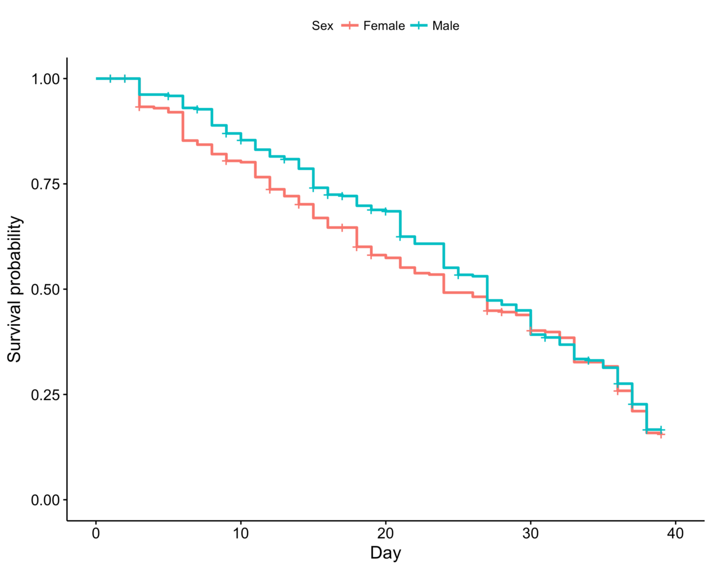
The first thing I looked at is age. We can see that early in the game, up to maybe day 27, males oftentimes last longer than females. This is quite an expected conclusion — the focus early on in the game, the tribal phase, is physical prowess, and males usually have an upper hand in this aspect. When tribes lose immunity challenges, they often target the least physically strong, which is sadly almost always women.
All in all, males tend to last longer than females as no strong reversal in the KM curves occurs.
Survival by Age
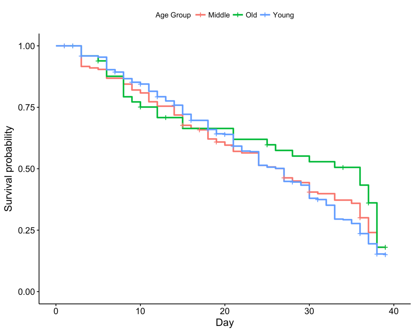
In terms of age, it’s interesting to see how young and old interchange on who lasts longer early and late in the game. In the early stage of the game, old castaways expectedly get voted out at a higher probability than young ones, and this reverses in the latter part of the game.
In other words, an old person has a higher chance of getting voted out early in the game compared to his younger peers, but if survives the first third of the game (up to about day 15), then he has a high chance of going deep in the game.
*By young, I mean someone aged between 18 to 35; by middle, 36 to 50; by old, above 50.


Survival by Age Group and Sex
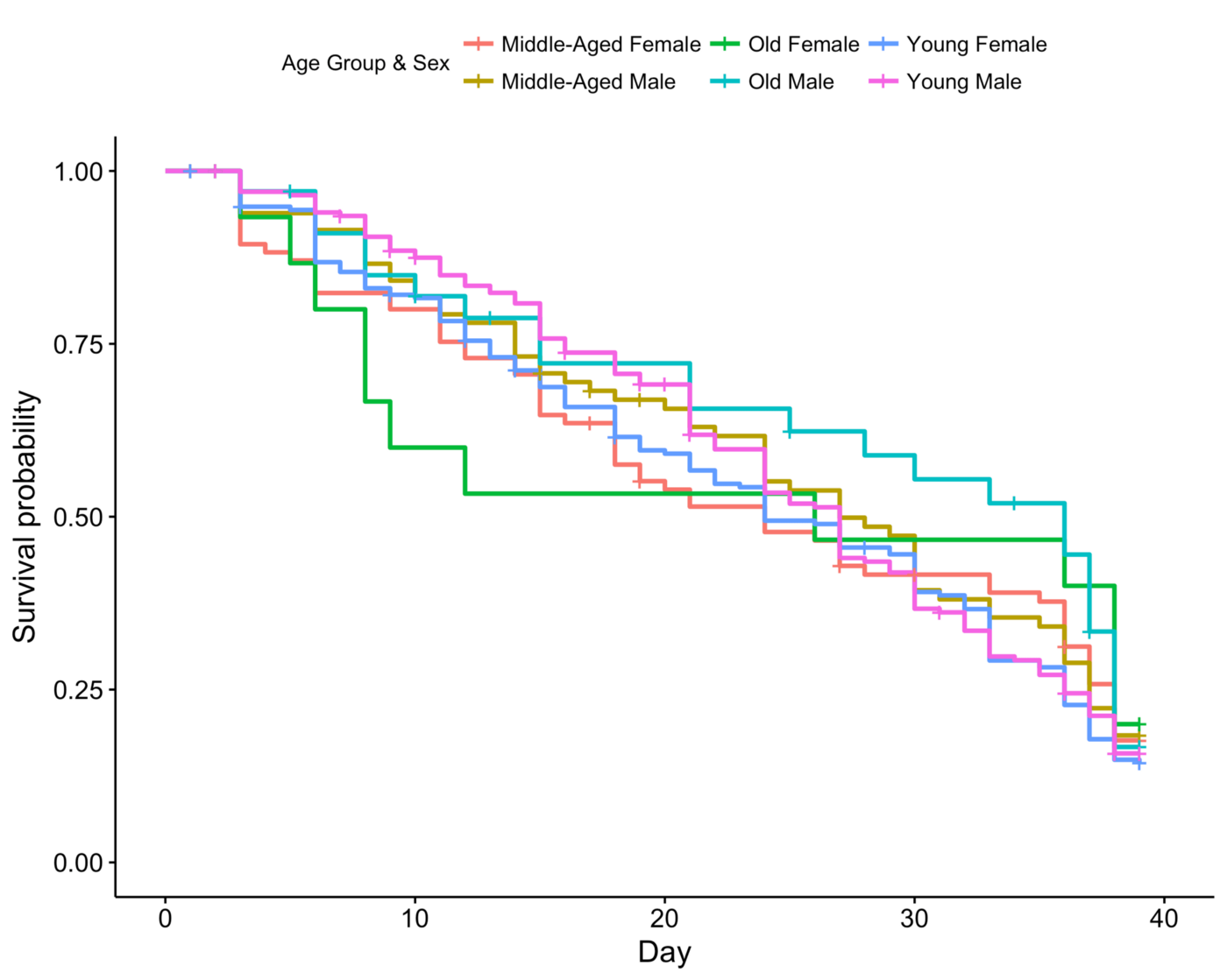
Let’s look at the combination of age and sex.
Old females expectedly get the short end of the stick in the early stage. So sorry, Sonja.
Young males have good survivability at the early stage but fall off as the game continues. They oftentimes get targeted as physical threats and are disposed off post-merge once their pre-merge challenge utility expires.

In terms of overall survivability, I’d say that old males have the best survival curve. They start out middle-of-the-pack in terms of survival probability in the early game, but once they get past merge, they tend to go deep in the game.
Survival by Region
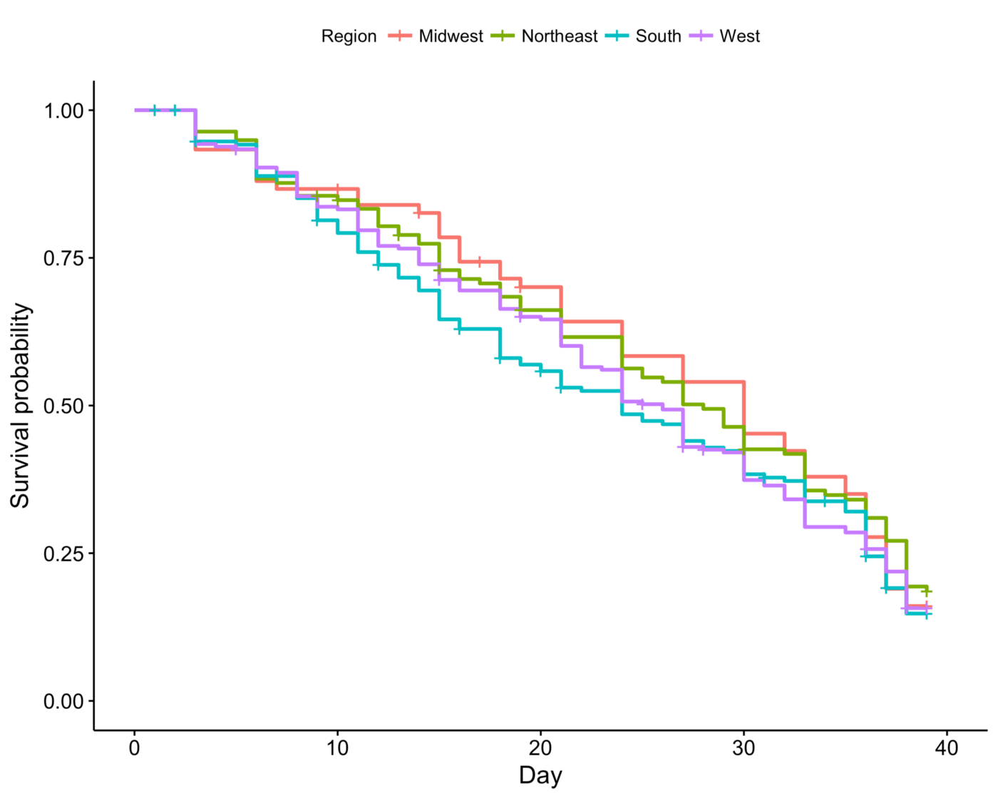
Now let’s look at the effect of geographic origin on the survival curves. Frankly, I’m not very knowledgeable about difference in culture across the four regions since I’m not from the US. Simply looking at the survival curves, we see that Midwest and South have the highest and lowest mid-game survivability, but Northeast leads in the endgame.
A Case for Old School vs. New School
If you’re a fan of the show, then you’re probably aware that Survivor can be split into Old School and New School in terms of the rigour of gameplay. Old School Survivor has more emphasis on survival, challenge prowess, no production twists, and less emphasis on hidden immunity idols. New School Survivor is the opposite - more emphasis is put on gameplay, hidden immunity idols, and shifting alliances.
The distinction of Old and New, when the former ended and the latter started, isn’t really set in stone. There’s actually a Reddit thread where people debate on where Old ends and New starts. The comment which I agree with the most is the one by PopsicleIncorporated, with Tocantins being the end of Old and Samoa being the start of New. That’s the division I’m going to use in all that follows.
The goal of this section is to see if there are significant differences in the survival curves for Old School and New School. Code can be accessed in my Github.
Survival by Sex
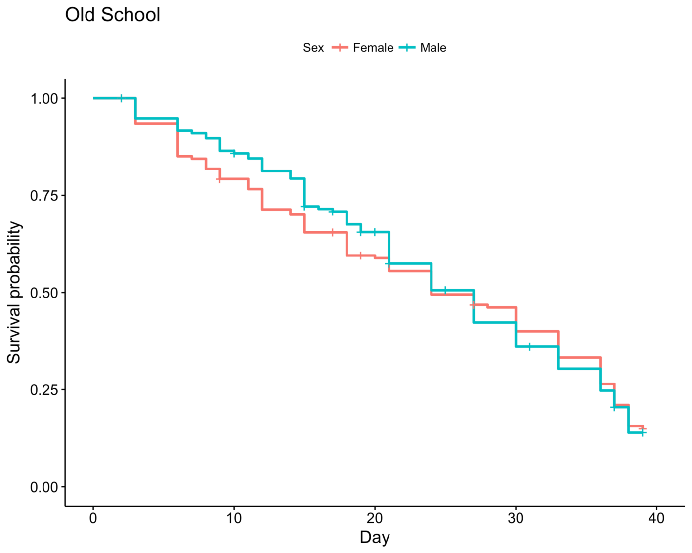 In Old School Survivor, there is a reversal between female and male on survivability. Early on, males have the upper hand, but it shifts around Day 27 onwards wherein females attain higher survivability.
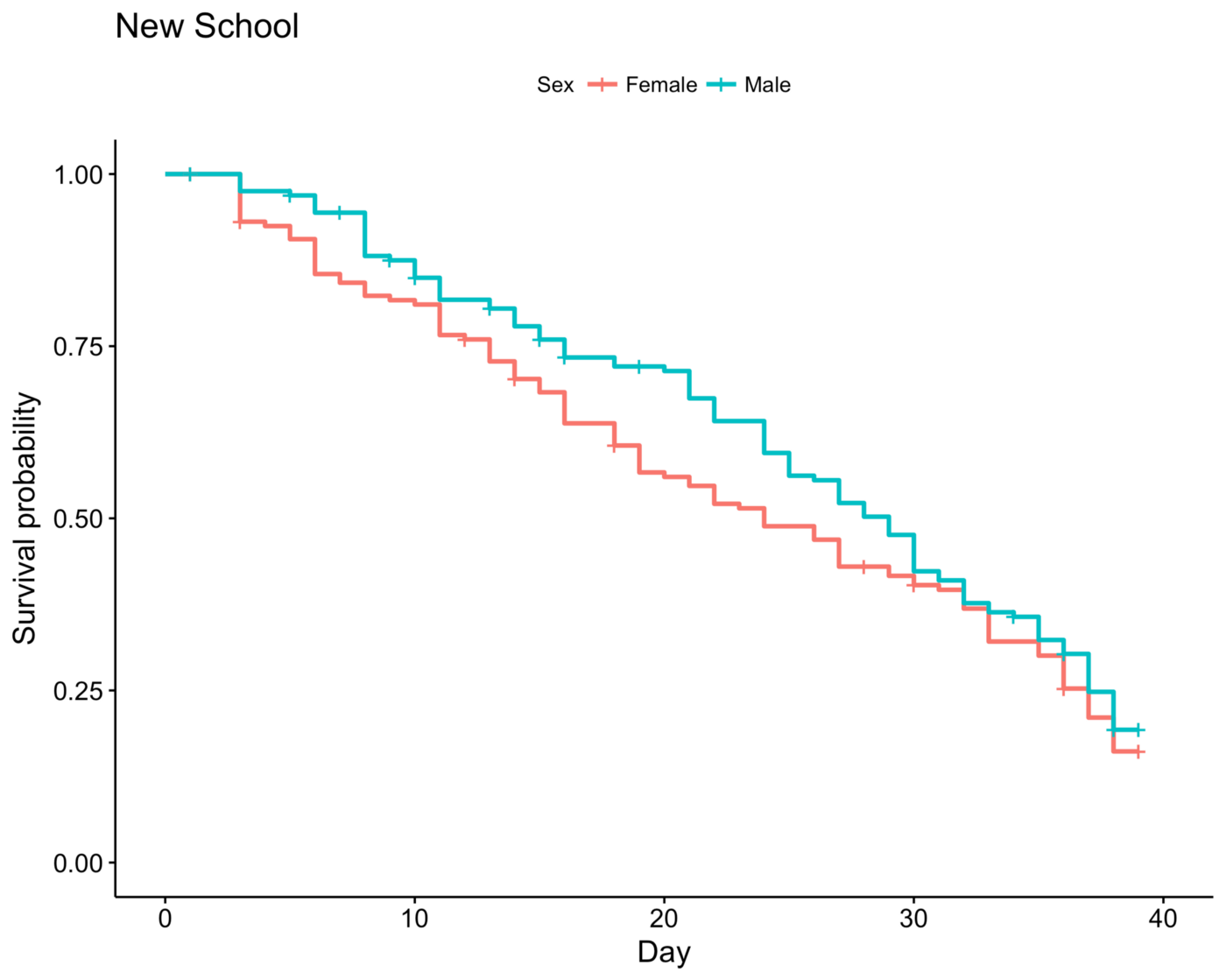 In the New School era, this reversal does not happen, and all throughout the game, males have higher survivability than females.
Survival by Age
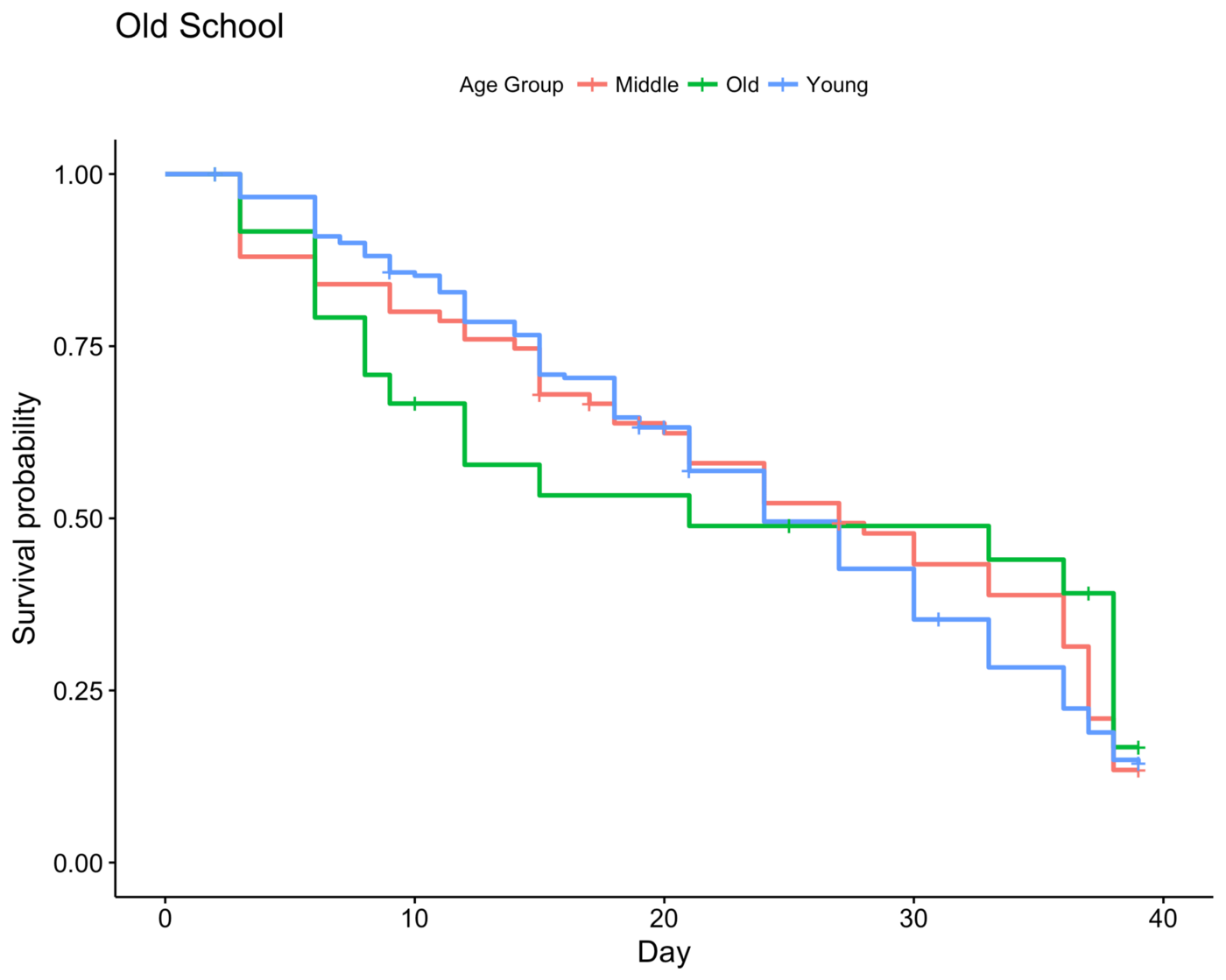 This is really interesting. In Old School Survivor, old people tend to have low survivability up until around Day 30 then it reverses after, similar to our observation in the baseline age analysis above…
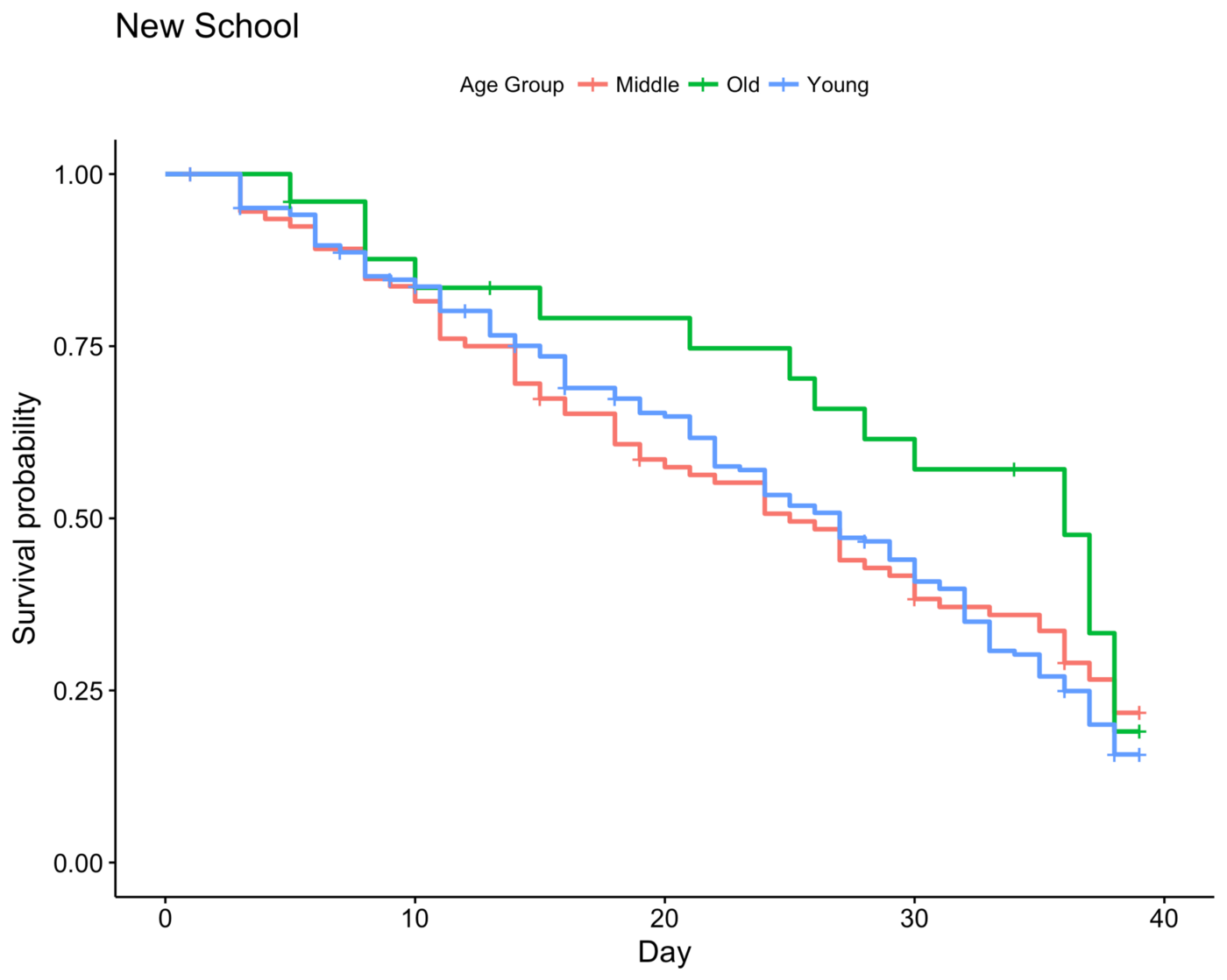 … while in New School Survivor, they tend to have high survivability overall.
One idea I have on this is that Old School Survivor tended to focus more on who is more deserving, and one of the main qualities that people tended to focus on was physical prowess and contribution to camp. By the nature of ageing, old castaways tend to have lower physicality and thus get voted out as a physical liability.
On the other hand, New School Survivor is much more strategic, where the focus shifts to eliminating threats — starting off with the physical threats when given the opportunity. Thus, old people are able to slip under the radar since they oftentimes are overshadowed by these threats. Age doesn’t factor in negatively in New School Survivor. In fact, it’s beneficial to be old since you’re viewed as a non-threat.

For the Future
There are a lot of things that can still be done with survival analysis on Survivor. All we have been doing is estimating the survival function with the Kaplan-Meier method. We haven’t really touched on statistical inference on survival rates. What we can do in the future is apply the Cox Proportional Hazards Model to see how the different demographic covariates relate with the hazard function, which can be interpreted as the instantaneous ‘risk’ of dying, opposite of what the survival function represents. Using the Cox PH model, we can quantify how age, sex, geography, and basically any variable affect the hazard of getting voted out (and in turn, the survivability).
But let’s save that topic for a rainy day.