

Black Mirror is interesting because it shows how things could go wrong if and when technology advances to the point wherein our morals as humans are challenged.
It’s not a secret that Black Mirror is super downbeat – the characters are usually broken people, the music is ominous, and the world it builds is generally gray. For a show that explores the dark side of modern tech, that’s to be expected. It was really hard for me to binge-watch the show since certain aspects of it are disturbing, but I couldn’t really keep my eyes off the TV. Can I use text analytics to obtain an objective ranking of the inherently subjective sentiment of Black Mirror episodes?
Browsing the Black Mirror thread of Reddit, I saw a lot of threads asking people to rank each Black Mirror episode according to how disturbing or depressing it is. Apart from how disturbing or how depressing the episodes are, another interesting thing to look at is the sentiment or mood of the episodes – how positive or negative are they? If one were to to rank episodes according to how downbeat and negative they are, what would the ranking look like?
Obviously, rankings are subjective and differ from person to person. This is precisely what’s interesting about rankings.
This made me think: Can I use text analytics to obtain an objective ranking of the inherently subjective sentiment of Black Mirror episodes? And if so, will I be able to justify the resulting ranking?
In this post, I utilize sentiment analysis to analyze Black Mirror episode subtitles, character dialog, and quantitatively assess their sentiment. From this analysis, I will be able to rank the episodes according to how negative they are. In actuality, since I’m analyzing dialog, what I’m actually dealing with is the sentiment of the characters.
By solely considering character dialog, I’m implicitly assuming that the sentiment of the episode is the sentiment of the characters; there are a lot of factors I am not considering, such as music and the visuals.
I use Python for this analysis. The full code can be accessed on Github. Here I use a specific lexical approach called VADER (Valence Aware Dictionary and sEntiment Reasoner), a lexicon and rule-based sentiment analysis tool. The nice thing about VADER is that it returns polarity scores in the range -1 to 1, most negative to most positive, respectively. This will enable us to rank texts according to their sentiment intensity. For more background on VADER, check out the last section of this blog post.
Conveniently, VADER has an open-source implementation in Python. This is what we’ll be using for this analysis.
Let’s now turn our attention to the data – what is it, where do we get it, and how can we analyze it?
Data Extraction and Processing
I used subtitle files from TV Subs as my text source. For each subtitle file, I did some pre-processing in order to return a single string which contains the whole dialog of the episode as a paragraph. Note that each subtitle file has time stamps, and so we need to remove these.
First, I loaded some dependencies, so these include text analysis functions as well as the base modules pandas and matplotlib. Then, I wrote a function return_dialog which takes as input the string name of the subtitle file and removes the time stamps to output the dialog as a single string.
# load dependencies
from vaderSentiment.vaderSentiment import SentimentIntensityAnalyzer
from nltk import tokenize
import pandas as pd
import matplotlib.pyplot as plt
import seaborn as sns
%matplotlib notebook

def return_dialog(sub):
    """
    Returns the dialog of the .srt file sub.
    Input :
        sub : name of the .srt file as a string, ex. 's01e01.srt'
    Output :
        dialog : dialog contained in .srt file as a single string
    """
    lines = []
    with open(sub) as file:
        # check the starting line of the dialog
        if sub == 'special.srt':
            start = 2
        elif int(sub[2]) == 1:
            start = 2
        elif int(sub[2]) == 2:
            start = 7
        else:
            start = 12
        for index,line in enumerate(file):
            if index >= start:
                # check if line contains dialog
                if (index == start) or ((index == start+1) and (len(line.split()) != 0)):
                    lines.append(line.strip('\n').replace('\'',''))
                    space_index = index
                if ((index > space_index + 2) and (len(line.split()) != 0)):
                    lines.append(line.strip('\n').replace('\'',''))
                if (len(line.split()) == 0):
                    space_index = index
    # output the dialog as a single string, removing the last two lines which contain attribution
    return ' '.join(lines[:-2])

# construct a list of string filenames for the subtitles
subs = ['s0'+str(i)+'e0'+str(j)+'.srt' for i in range(1,4) for j in range(1,4)]
subs = subs + ['s03e0' + str(k)+'.srt' for k in range(4,7)]
subs.insert(6,'special.srt')
Next, I tried to obtain the VADER polarity score of each whole subtitle file as a whole. This didn’t work that well since the returning scores were around -1 and 1, which are the minimum and maximum values. It seems that VADER doesn’t really work that well when evaluating the polarity of very large texts.
# call the VADER analysis object
analyzer = SentimentIntensityAnalyzer()

pols = []
for sub in subs:
    di = return_dialog(sub)
    pols.append(analyzer.polarity_scores(di)['compound'])
print(pols)
Applying VADER on the whole dialog doesn’t really work out. Because of this, I resorted to, instead, apply VADER on a sentence level. To split the paragraph into a list of sentences, I used the NLTK sentence tokenizer tokenize.sent_tokenize(). The polarity score of the whole dialog, in this case, is the average of the polarity scores of its individual sentences. To make analysis easier, I built a pandas data frame of sentences, wherein the column data consist of the episode name, subtitle file name, polarity score, and whether it is a positively labeled sentence or a negatively labeled sentence. A positively labeled sentence is defined as one which has a positive VADER polarity score.
Note that there are a lot of sentences without sentiment, i.e. having polarity score zero. Including these causes the mean polarity to be almost zero. I decided to ignore non-sentiment-bearing sentence in the analysis.
# build a dictionary of sub name to episode title
names = {
    subs[0]: 'The National Anthem',
    subs[1]: 'Fifteen Million Merits',
    subs[2]: 'The Entire History of You',
    subs[3]: 'Be Right Back',
    subs[4]: 'White Bear',
    subs[5]: 'The Waldo Moment',
    subs[6]: 'White Christmas',
    subs[7]: 'Nosedive',
    subs[8]: 'Playtest',
    subs[9]: 'Shut Up and Dance',
    subs[10]: 'San Junipero',
    subs[11]: 'Men Against Fire',
    subs[12]: 'Hated in the Nation'
}

# rows will contain the rows of the data frame containing the sentences in
# each subtitle file
rows = []

for sub in subs:
    print(sub)
    di = return_dialog(sub)
    sen = tokenize.sent_tokenize(di)
    for s in sen:
        pol = analyzer.polarity_scores(s)['compound']
        # check if sentence s has sentiment/ nonzero polarity
        if pol != 0:
            # check the polarity of the sentence.
            # append a dictionary with info regarding the sentence into rows
            rows.append({'Episode': sub, 'Name': names[sub], 'Sentence':s,
                         'Score': pol, 'isPos': pol>0})

# convert the rows into a dataframe for easier plotting and analysis
df = pd.DataFrame(rows)

print(df.head())
From the data frame, we can easily plot the data for each episode. The following code plots a swarmplot and a violinplot for each episode in Season 1. The same can be done for other seasons.
# plot a violinplot and swarmplot for each episode

# plot first season episodes
plt.close()
plt.figure(figsize=(10,5))
plt.ylim(-1.2,1.2)
sns.violinplot(x='Name',y='Score',data=df[df['Episode'].isin(subs[:3])],inner=None)
sns.swarmplot(x="Name", y="Score",data=df[df['Episode'].isin(subs[:3])], color="black", alpha=.9);
plt.xlabel('')
plt.xticks(size=12)
plt.ylabel('VADER Compound Sentiment Score',size=15)
plt.savefig('Season1.png')
Sentiment Analysis of Black Mirror S1-S3
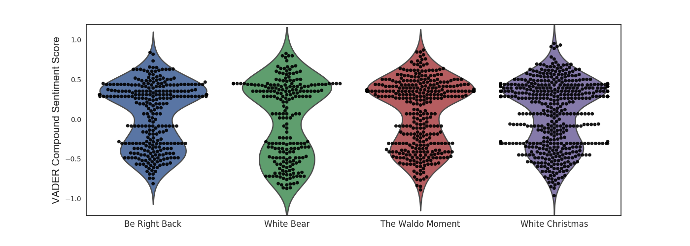
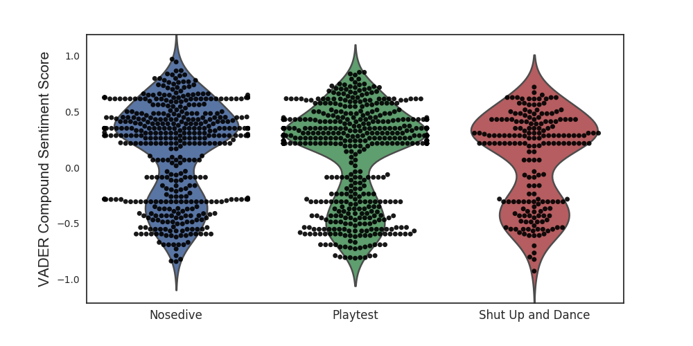
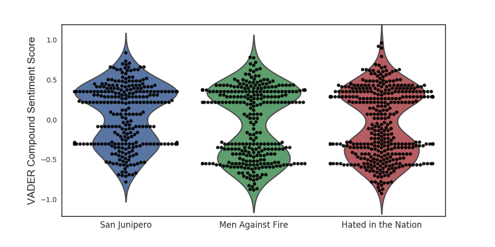
After constructing a data frame of sentences per episode and their associated VADER polarity scores, we can use the Seaborn library in Python to visualize the sentiment distribution, the distribution of polarity scores, per episode. Below are plots that show just that. These plots are actually two superimposed plots – a swarmplot (aka the dots) and a violinplot (aka the smooth outer layer).
Swarmplots are similar to histograms in the way that they show the distribution of scores. The larger the number of dots corresponding to a polarity score, the higher the number of sentences with that polarity score. Violinplots, on the other hand, show the kernel density estimate (KDE) of the data. Intuitively, this is a smooth estimate of the underlying distribution of the data.
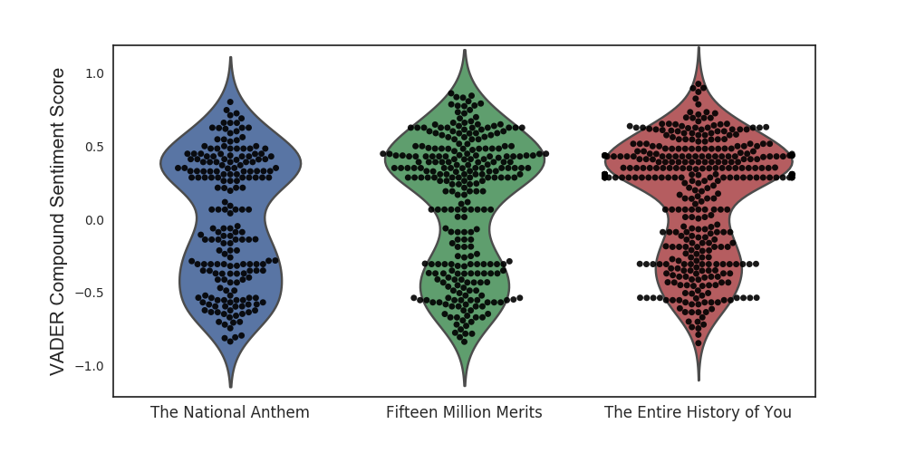
Note that the KDE plots actually extend beyond the -1 to 1 range. This is because KDE does not recognize the sentiment range; its aim is to smooth out the data and approximate the underlying distribution. Actually, I only drew the KDE in order to make the shapes of the sentiment distributions more apparent.
After admiring how cute the plots are, we can see that all of them show a bimodal distribution – one peak at a positive score and another at a negative score. What is interesting to see is which peak actually dominates – the positive or the negative? For some episodes, like The Entire History of You, Nosedive, and the Waldo Moment, the positive peak clearly dominates; while for some, like The National Anthem and Hated in the Nation, it’s less obvious.
We can quantitatively compare the episodes by comparing the means of the underlying sentiment distributions. We consider three different means:
- mean polarity score of the positively labeled sentences : MP
- mean polarity score of the negatively labeled sentences: MN
- mean of the sentiment distribution: MA
The mean polarity score of the positively labeled sentences (MP) only considers the positively labeled sentences, that is, the sentences which have VADER polarity that is positive. MP quantifies the intensity of the positive sentences in the script, without regard for the negative ones. The interpretation of the mean polarity score of the negatively labeled sentences (MN) is analogous to this, with positive and negative interchanged.
On the other hand, the mean of the sentiment distribution (MA) is the mean polarity of all sentiment-bearing sentences, which includes both positive and negative. Note that when calculating MA, we are adding a bunch of positive quantities and negative quantities, so we most likely end up with a number near zero, if the positive and negative are evenly matched. We can interpret MA as a quantity which characterizes the overall sentiment of the episode – with the sign containing information on which sentiment, positive or negative, prevailed.
Again, as I’ve mentioned earlier, we are using the sentiment of character dialog as a proxy for the sentiment of the episode. A lot of important things – such as the audio and visuals – are not included. It’s best to keep that in mind.
We can obtain these rankings using a simple group-by on the data frame of episodes.
# rank the episodes according to the mean polarity score of their positive sentences (MP)
df[df['isPos']].groupby('Name')['Score'].mean().sort_values()

# rank the episodes according to the mean polarity score of their negative sentences (MN)
df[~df['isPos']].groupby('Name')['Score'].mean().sort_values()

# rank the episodes according to the mean of their sentiment distribution (MA)
df.groupby('Name')['Score'].mean().sort_values()
To add some excitement, let’s first look at how the episodes rank with respect to the mean polarity score of the positively labeled sentences (MP) and the mean polarity score of the negatively labeled sentences (MN). Let’s save the ranking with respect to the mean of the sentiment distribution (MA), which represents an overall ranking, for last.
Intensity of Positive Moments
First, let’s look at how the episodes rank with respect to the mean polarity score of the positively labeled sentences (MP). This ranking answers the question: How (positively) intense are the positive moments?
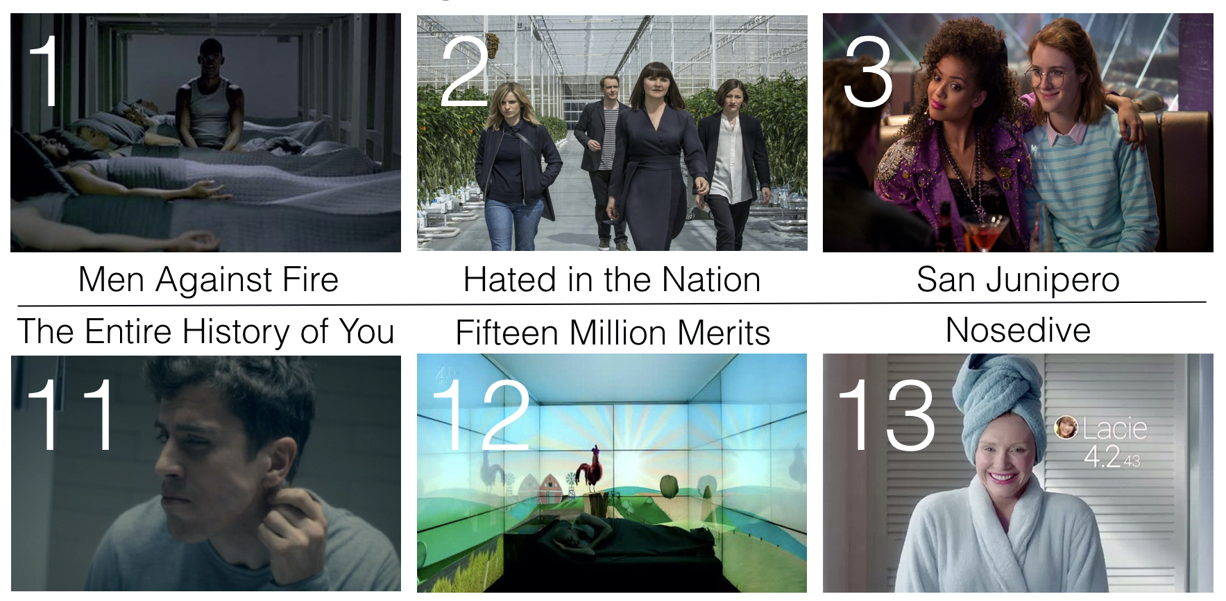
Men Against Fire, the episode on population cleansing, and Hated in the Nation, the episode on killer bees, appear at the top of the ranking. This means that when these episodes are positive, they’re just mildly so. Thinking about it, it is not really that surprising to see these two episodes at the top since their storylines and characters are completely downbeat, with no real happy moments, as far as I can remember. The appearance of San Junipero at third place is quite surprising to me. After watching the episode, I felt that the it was really positive. Well, maybe the ending just made me feel that way?
Nosedive appearing at the bottom is really expected since its world, wherein people ‘rate’ each other according to perception, demands that citizens be superficially cheery. Lacie Pound, the main character of Nosedive, is the embodiment of sunshine from the start of the episode up until before the very end. Fifteen Million Merits makes an appearance at the second from the bottom. Because the episode revolves around a talent show, which is a lot of fun (until that moment with Abi!) and a love link between its two leads, it is justifiable why it appears near the bottom. The rank of Entire History of You is also expected since a large chunk of the episode is set at a lively dinner party.
Intensity of Negative Moments
Next, let’s look at at how the episodes rank with respect to the mean polarity score of the negatively labeled sentences (MP). This ranking answers the question: How (negatively) intense are the negative moments?
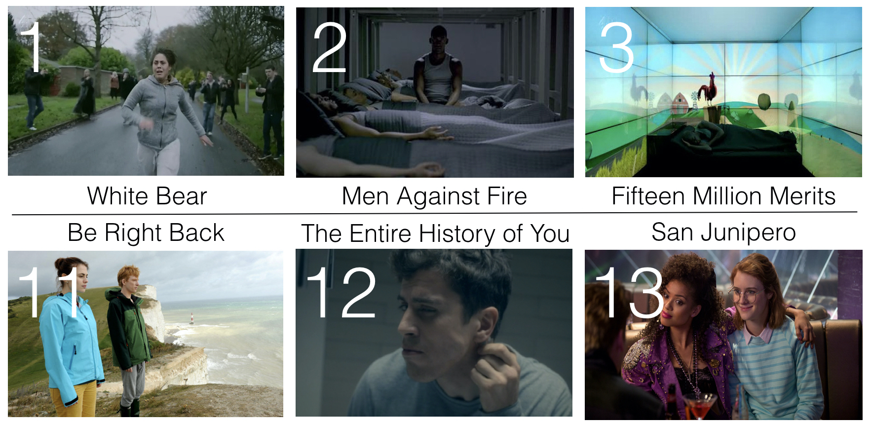
I completely agree with White Bear being at the top of the list. When the episode is upsetting, it is REALLY upsetting. Victoria Skillane, the protagonist, is a sympathetic monster. However, the punishment that she faces due to her crime is inhumane, and it reflects on society as well. Again, Men Against Fire appears at the top. Fifteen Million Merits appears at the third place. This is interesting, given that in the ranking for MP, it appears near the bottom. This means that when Fifteen Million Merits is positive, it’s really positive; when it’s negative, it’s really negative. Even though the show revolves around a fun talent show, it doesn’t take long before it shows its dark underbelly.
The bottom three are San Junipero, The Entire History of You, and Be Right Back. The presence of San Junipero at the bottom is justified, since there aren’t really any very upsetting or disturbing things that happened in the episode. The episode simply focuses on a love story that we can all get behind. The placing of The Entire History of You is quite interesting. I expected it to appear higher in the MN ranking. The scenes leading to the ending are quite upsetting. I only used the dialog of the show’s characters as the basis, maybe this isn’t captured? Be Right Back’s placing is understandable. The sad parts of the episode are mild compared to the other episodes.
Overall (Negative) Polarity
Now, let’s look at the overall ranking – the ranking with respect to the mean of the sentiment distribution (MA):
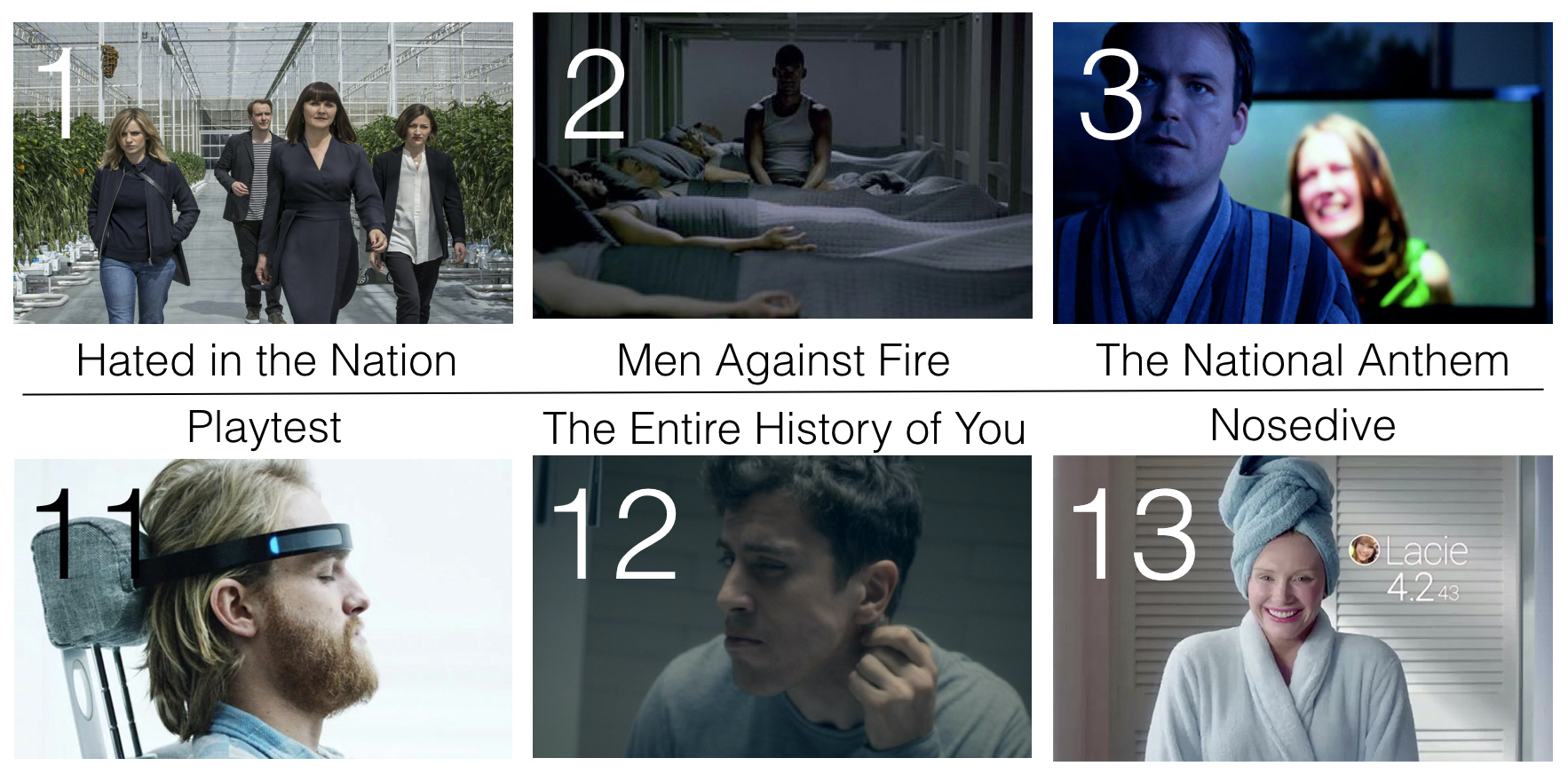
It is interesting to see that Hated in the Nation and Men Against Fire, the last two episodes of the series, appear at the top of the list and are the only ones that have a negative MA score. This means that, overall, these episodes have the most negative sentiment. Well, apparently, the writer of the show, Charlie Brooker, really knows how to end with a bang! It’s not really difficult to see why these two are at the top. They’re just really sad and negative episodes, plain and simple. The National Anthem appearing in third place is expected as well. Even though there are subtle comedic elements, the episode is pretty gray overall.
On the other hand, it is not really surprising to see Nosedive at the bottom of the list. Basically, the lead, Lacie Pound, is happiness incarnate. The Entire History of You in second place is quite unexpected. Playtest’s position in third isn’t questionable. The episode’s lead, Cooper, is a very cheery and outgoing man, and imparts a lot of positivity to the episode.
The only thing I didn’t really expect is for San Junipero to appear around the middle – I expected it to appear near the bottom. Overall, I found the episode to be positive. Again, maybe it’s just because of the ending?
Final Thoughts: Black Mirror + VADER
Overall, the rankings I obtained are quite reasonable. I think VADER is a legit tool to analyze sentiment at the sentence level. However, this analysis is really, really basic – a lot of things can be done to improve it.
There are a lot of factors which affect negativity not included here. Primarily, the audio and the visuals. More complicated tools, such as audio and image processing can be used to include these factors in the analysis. However, I do not have these tools up in my arsenal as of this moment.
Originally, I wanted to do a ranking of how depressing each Black Mirror episode is, but I realized that this is difficult to quantify. I do not really know of any metric to quantify this emotion. In lieu, I resorted to ranking the episodes according to how downbeat or negative they are.
It would also be interesting to see how the results would change with a different algorithm. There’s an open source implementation of Textblob in Python.
A project that I intend to do is to look at the sentiment of each episode over time. As each episode – well, in Seasons 1 and 2 anyway – is divided into acts, it would be interesting to see the progression of sentiment across acts.
A Primer on VADER
Read on if you’re interested to learn how VADER works under the hood.
VADER (Valence Aware Dictionary for sEntiment Reasoning) is a model used for sentiment analysis that is sensitive to both polarity (positive/negative) and intensity (strength) of emotion. Introduced in 2014, VADER sentiment analysis uses a human-centric approach, combining qualitative analysis and empirical validation by using human raters and the wisdom of the crowd.
In this footnote, I’ll discuss how VADER calculates the valence score of an input text. It combines a dictionary, which maps lexical features to emotion intensity, and five simple heuristics, which encode how contextual elements increment, decrement, or negate the sentiment of text.
Before doing that, let’s go one level above and talk about sentiment analysis in general.
(Access the VADER paper here.)
What is Sentiment Analysis?
Consider the following sentences:
The party is wonderful.
I hate that man.
Do you get a sense of the feelings that these sentences imply? The first one clearly conveys positive emotion, whereas the second conveys negative emotion. Humans associate words, phrases, and sentences with emotion. The field of Sentiment Analysis attempts to use computational algorithms in order to decode and quantify the emotion contained in media such as text, audio, and video.
Sentiment Analysis is a really big field with a lot of academic literature behind it. However, its tools really just boil down to two approaches: the lexical approach and the machine learning approach.
Lexical approaches aim to map words to sentiment by building a lexicon or a ‘dictionary of sentiment.’ We can use this dictionary to assess the sentiment of phrases and sentences, without the need of looking at anything else. Sentiment can be categorical – such as {negative, neutral, positive} – or it can be numerical – like a range of intensities or scores. Lexical approaches look at the sentiment category or score of each word in the sentence and decide what the sentiment category or score of the whole sentence is. The power of lexical approaches lies in the fact that we do not need to train a model using labeled data, since we have everything we need to assess the sentiment of sentences in the dictionary of emotions. VADER is an example of a lexical method.
Machine learning approaches, on the other hand, look at previously labeled data in order to determine the sentiment of never-before-seen sentences. The machine learning approach involves training a model using previously seen text to predict/classify the sentiment of some new input text. The nice thing about machine learning approaches is that, with a greater volume of data, we generally get better prediction or classification results. However, unlike lexical approaches, we need previously labeled data in order to actually use machine learning models.
Quantifying the Emotion of a Word
Primarily, VADER relies on a dictionary which maps lexical features to emotion intensities called valence scores. The valence score of a text can be obtained by summing up the intensity of each word in the text.
What is a lexical feature? How do we even measure emotional intensity?
By lexical feature, I mean anything that we use for textual communication. Think of a tweet as an example. In a typical tweet, we can find not only words, but also emoticons like “:-)”, acronyms like “LOL”, and slang like “meh”. The cool thing about VADER is that these colloquialisms get mapped to intensity values as well.
Emotion intensity or valence score is measured on a scale from -4 to +4, where -4 is the most negative and +4 is the most positive. The midpoint 0 represents a neutral sentiment. Sample entries in the dictionary are “horrible” and “okay,” which get mapped to -2.5 and 0.9, respectively. In addition, the emoticons “/-:” and “0:-3” get mapped to -1.3 and 1.5.
The next question is, how do we construct this dictionary?
By using human raters from Amazon Mechanical Turk!
Ok. You might be thinking that emotional intensity can be very arbitrary since it depends on who you ask. Some words might not seem very negative to you, but they might be to me. To counter this, the creators of VADER enlisted not just one, but a number of human raters and averaged their ratings for each word. This relies on the concept of the wisdom of the crowd : collective opinion is oftentimes more trustworthy than individual opinion. Think of the game show “Who Wants to Be a Millionaire?” One of the lifelines that contestants can use is Ask the Audience, which also relies on the wisdom of the crowd.
Quantifying the Emotion of a Sentence
VADER (well, in the Python implementation anyway) returns a valence score in the range -1 to 1, from most negative to most positive.
The valence score of a sentence is calculated by summing up the valence scores of each VADER-dictionary-listed word in the sentence. Cautious readers would probably notice that there is a contradiction: individual words have a valence score between -4 to 4, but the returned valence score of a sentence is between -1 to 1.
They’re both true. The valence score of a sentence is the sum of the valence score of each sentiment-bearing word. However, we apply a normalization to the total to map it to a value between -1 to 1.
The normalization used by Hutto is
where x is the sum of the valence scores of the constituent words of the sentence and alpha is a normalization parameter that we set to 15. The normalization is graphed below.
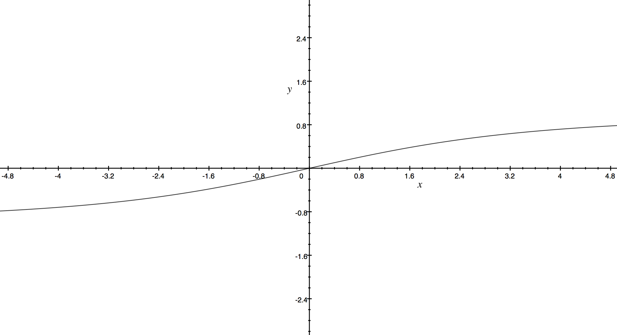
We see here that as x grows larger, it gets more and more close to -1 or 1. To similar effect, if there are a lot of words in the document you’re applying VADER sentiment analysis to, you get a score close to -1 or 1. Thus, VADER works best on short documents, like tweets and sentences, not on large documents.
Five Simple Heuristics
Lexical features aren’t the only things in the sentence which affect the sentiment. There are other contextual elements, like punctuation, capitalization, and modifiers which also impart emotion. VADER takes these into account by considering five simple heuristics. The effect of these heuristics are, again, quantified using human raters.

The first heuristic is punctuation. Compare “I like it.” and “I like it!!!” It’s not really hard to argue that the second sentence has more intense emotion than the first, and therefore must have a higher VADER valence score.
VADER takes this into account by amplifying the valence score of the sentence proportional to the number of exclamation points and question marks ending the sentence. VADER first computes the valence score of the sentence. If the score is positive, VADER adds a certain empirically-obtained quantity for every exclamation point (0.292) and question mark (0.18). If the score is negative, VADER subtracts.
The second heuristic is capitalization. “AMAZING performance.” is definitely more intense than “amazing performance.” And so VADER takes this into account by incrementing or decrementing the valence score of the word by 0.733, depending on whether the word is positive or negative, respectively.

The third heuristic is the use of degree modifiers. Take for example “effing cute” and “sort of cute”. The effect of the modifier in the first sentence is to increase the intensity of cute, while in the second sentence, it is to decrease the intensity. VADER maintains a booster dictionary which contains a set of boosters and dampeners.
The effect of the degree modifier also depends on its distance to the word it’s modifying. Farther words have a relatively smaller intensifying effect on the base word. One modifier beside the base word adds or subtracts 0.293 to the valence score of the sentence, depending on whether the base word is positive or not. A second modifier from the base word adds/subtracts 95% of 0.293, and a third adds/subtracts 90%.

The fourth heuristic is the shift in polarity due to “but”. Oftentimes, “but” connects two clauses with contrasting sentiments. The dominant sentiment, however, is the latter one. For example, “I love you, but I don’t want to be with you anymore.” The first clause “I love you” is positive, but the second one “I don’t want to be with you anymore.” is negative and obviously more dominant sentiment-wise.
VADER implements a “but” checker. Basically, all sentiment-bearing words before the “but” have their valence reduced to 50% of their values, while those after the “but” increase to 150% of their values.
The fifth heuristic is examining the tri-gram before a sentiment-laden lexical feature to catch polarity negation. Here, a tri-gram refers to a set of three lexical features. VADER maintains a list of negator words. Negation is captured by multiplying the valence score of the sentiment-laden lexical feature by an empirically-determined value -0.74.
VADER Sentiment Analysis Wrap Up
VADER combines a dictionary of lexical features to valence scores with a set of five heuristics. The model works best when applied to social media text, but it has also proven itself to be a great tool when analyzing the sentiment of movie reviews and opinion articles.